sensorsig
Simulate received signal at sensor array
Syntax
Description
x = sensorsig(pos,ns,ang)pos represents
the positions of the array elements, each of which is assumed to be
isotropic. ns indicates the number of snapshots
of the simulated signal. ang represents the incoming
directions of each plane wave signal. The plane wave signals are assumed
to be constant-modulus signals with random phases.
Examples
Simulate the received signal at an array, and use the data to estimate the arrival directions.
Create an 8-element uniform linear array whose elements are spaced half a wavelength apart.
fc = 3e8;
c = 3e8;
lambda = c/fc;
array = phased.ULA(8,lambda/2);
Simulate 100 snapshots of the received signal at the array. Assume there are two signals, coming from azimuth 30° and 60°, respectively. The noise is white across all array elements, and the SNR is 10 dB.
x = sensorsig(getElementPosition(array)/lambda,...
   100,[30 60],db2pow(-10));
Use a beamscan spatial spectrum estimator to estimate the arrival directions, based on the simulated data.
estimator = phased.BeamscanEstimator('SensorArray',array,...
   'PropagationSpeed',c,'OperatingFrequency',fc,...
   'DOAOutputPort',true,'NumSignals',2);
[~,ang_est] = estimator(x);
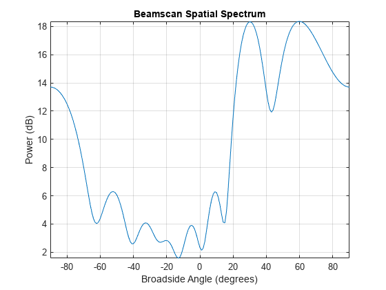
Plot the spatial spectrum resulting from the estimation process.
plotSpectrum(estimator)

The plot shows peaks at 30° and 60°.
Simulate receiving two uncorrelated incoming signals that have different power levels. A vector named scov stores the power levels.
Create an 8-element uniform linear array whose elements are spaced half a wavelength apart.
fc = 3e8;
c = 3e8;
lambda = c/fc;
ha = phased.ULA(8,lambda/2);
Simulate 100 snapshots of the received signal at the array. Assume that one incoming signal originates from 30 degrees azimuth and has a power of 3 W. A second incoming signal originates from 60 degrees azimuth and has a power of 1 W. The two signals are not correlated with each other. The noise is white across all array elements, and the SNR is 10 dB.
ang = [30 60];
scov = [3 1];
x = sensorsig(getElementPosition(ha)/lambda,...
   100,ang,db2pow(-10),scov);
Use a beamscan spatial spectrum estimator to estimate the arrival directions, based on the simulated data.
hdoa = phased.BeamscanEstimator('SensorArray',ha,...
   'PropagationSpeed',c,'OperatingFrequency',fc,...
   'DOAOutputPort',true,'NumSignals',2);
[~,ang_est] = step(hdoa,x);
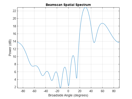
Plot the spatial spectrum resulting from the estimation process.
plotSpectrum(hdoa);

The plot shows a high peak at 30 degrees and a lower peak at 60 degrees.
Simulate the reception of three signals, two of which are correlated.
Create a signal covariance matrix in which the first and third of three signals are correlated with each other.
scov = [1 0 0.6;...
        0 2 0;...
        0.6 0 1];
Simulate receiving 100 snapshots of three incoming signals from 30°, 40°, and 60° azimuth, respectively. The array that receives the signals is an 8-element uniform linear array whose elements are spaced one-half wavelength apart. The noise is white across all array elements, and the SNR is 10 dB.
pos = (0:7)*0.5;
ns = 100;
ang = [30 40 60];
ncov = db2pow(-10);
x = sensorsig(pos,ns,ang,ncov,scov);
Simulate receiving a signal at a URA. Compare the signal theoretical covariance with its sample covariance.
Create a 2-by-2 uniform rectangular array having elements spaced 1/4-wavelength apart.
pos = 0.25 * [0 0 0 0; -1 1 -1 1; -1 -1 1 1];
Define the noise power independently for each of the four array elements. Each entry in ncov is the noise power of an array element. This element position is the corresponding column in pos. Assume the noise is uncorrelated across elements.
ncov = db2pow([-9 -10 -10 -11]);
Simulate 100 snapshots of the received signal at the array, and store the theoretical and empirical covariance matrices. Assume that one incoming signal originates from 30° azimuth and 10° elevation. A second incoming signal originates from 50° azimuth and 0° elevation. The signals have a power of 1 W and are uncorrelated.
ns = 100;
ang1 = [30; 10];
ang2 = [50; 0];
ang = [ang1, ang2];
rng default
[x,rt,r] = sensorsig(pos,ns,ang,ncov);
View the magnitudes of the theoretical covariance and sample covariance.
abs(rt)
ans = 4×4

    2.1259    1.8181    1.9261    1.9754
    1.8181    2.1000    1.5263    1.9261
    1.9261    1.5263    2.1000    1.8181
    1.9754    1.9261    1.8181    2.0794
abs(r)
ans = 4×4

    2.2107    1.7961    2.0205    1.9813
    1.7961    1.9858    1.5163    1.8384
    2.0205    1.5163    2.1762    1.8072
    1.9813    1.8384    1.8072    2.0000
Simulate receiving a signal at a ULA, where the noise between different sensors is correlated.
Create a 4-element uniform linear array whose elements are spaced one-half wavelength apart.
pos = 0.5 * (0:3);
Define the noise covariance matrix. The value in the ( k,_j_) position in the ncov matrix is the covariance between the k and j array elements listed in array.
ncov = 0.1 * [1 0.1 0 0; 0.1 1 0.1 0; 0 0.1 1 0.1; 0 0 0.1 1];
Simulate 100 snapshots of the received signal at the array. Assume that one incoming signal originates from 60° azimuth.
ns = 100;
ang = 60;
[x,rt,r] = sensorsig(pos,ns,ang,ncov);
View the theoretical and sample covariance matrices for the received signal.
rt,r
rt = 4×4 complex

   1.1000 + 0.0000i  -0.9027 - 0.4086i   0.6661 + 0.7458i  -0.3033 - 0.9529i
  -0.9027 + 0.4086i   1.1000 + 0.0000i  -0.9027 - 0.4086i   0.6661 + 0.7458i
   0.6661 - 0.7458i  -0.9027 + 0.4086i   1.1000 + 0.0000i  -0.9027 - 0.4086i
  -0.3033 + 0.9529i   0.6661 - 0.7458i  -0.9027 + 0.4086i   1.1000 + 0.0000i
r = 4×4 complex

   1.1059 + 0.0000i  -0.8681 - 0.4116i   0.6550 + 0.7017i  -0.3151 - 0.9363i
  -0.8681 + 0.4116i   1.0037 + 0.0000i  -0.8458 - 0.3456i   0.6578 + 0.6750i
   0.6550 - 0.7017i  -0.8458 + 0.3456i   1.0260 + 0.0000i  -0.8775 - 0.3753i
  -0.3151 + 0.9363i   0.6578 - 0.6750i  -0.8775 + 0.3753i   1.0606 + 0.0000i
Input Arguments
Positions of elements in sensor array, specified as an N-column
vector or matrix. The values in the matrix are in units of signal
wavelength. For example, [0 1 2] describes three
elements that are spaced one signal wavelength apart. N is the number
of elements in the array.
Dimensions of pos:
For a linear array along the y axis, specify the y coordinates of the elements in a 1-by-N vector.
For a planar array in the yz plane, specify the y and z coordinates of the elements in columns of a 2-by-N matrix.
For an array of arbitrary shape, specify the x, y, and z coordinates of the elements in columns of a 3-by-N matrix.
Data Types: double
Number of snapshots of simulated signal, specified as a positive integer scalar. The function returns this number of samples per array element.
Data Types: double
Directions of incoming plane wave signals, specified as an M-column vector or matrix in degrees. M is the number of incoming signals.
Dimensions of ang:
If
angis a 2-by-M matrix, each column specifies a direction. Each column is in the form[azimuth; elevation]. The azimuth angle must be between –180 and 180 degrees, inclusive. The elevation angle must be between –90 and 90 degrees, inclusive.If
angis a 1-by-M vector, each entry specifies an azimuth angle. In this case, the corresponding elevation angle is assumed to be 0.
Data Types: double
Noise characteristics, specified as a nonnegative scalar, 1-by-N vector of positive numbers, or N-by-N positive definite matrix.
Dimensions of ncov:
If
ncovis a scalar, it represents the noise power of the white noise across all receiving sensor elements, in watts. In particular, a value of0indicates that there is no noise.If
ncovis a 1-by-N vector, each entry represents the noise power of one of the sensor elements, in watts. The noise is uncorrelated across sensors.If
ncovis an N-by-N matrix, it represents the covariance matrix for the noise across all sensor elements.
Data Types: double
Incoming signal characteristics, specified as a positive scalar, 1-by-M vector of positive numbers, or M-by-M positive semidefinite matrix.
Dimensions of scov:
If
scovis a scalar, it represents the power of all incoming signals, in watts. In this case, all incoming signals are uncorrelated and share the same power level.If
scovis a 1-by-M vector, each entry represents the power of one of the incoming signals, in watts. In this case, all incoming signals are uncorrelated with each other.If
scovis an M-by-M matrix, it represents the covariance matrix for all incoming signals. The matrix describes the correlation among the incoming signals. In this case,scovcan be real or complex.
Data Types: double
Array element taper, specified as a scalar or complex-valued N-by-1
column vector. The dimension N is the number of
array elements. If taper is a scalar, all elements
in the array use the same value. If taper is
a vector, each entry specifies the taper applied to the corresponding
array element.
Data Types: double
Complex Number Support: Yes
Output Arguments
Received signal at sensor array, returned as a complex ns-by-N
matrix. Each column represents the received signal at the corresponding
element of the array. Each row represents a snapshot.
Theoretical covariance matrix of the received signal, returned as a complex N-by-N matrix.
More About
The azimuth angle of a vector is the angle between the x-axis and the orthogonal projection of the vector onto the xy plane. The angle is positive in going from the x axis toward the y axis. Azimuth angles lie between –180 and 180 degrees. The elevation angle is the angle between the vector and its orthogonal projection onto the xy-plane. The angle is positive when going toward the positive z-axis from the xy plane. By default, the boresight direction of an element or array is aligned with the positive x-axis. The boresight direction is the direction of the main lobe of an element or array.
Note
The elevation angle is sometimes defined in the literature as the angle a vector makes with the positive z-axis. The MATLAB® and Phased Array System Toolbox™ products do not use this definition.
This figure illustrates the azimuth angle and elevation angle for a vector shown as a green solid line.

Extended Capabilities
Usage notes and limitations:
Does not support variable-size inputs.
Version History
Introduced in R2012b
See Also
MATLAB Command
You clicked a link that corresponds to this MATLAB command:
Run the command by entering it in the MATLAB Command Window. Web browsers do not support MATLAB commands.
웹사이트 선택
번역된 콘텐츠를 보고 지역별 이벤트와 혜택을 살펴보려면 웹사이트를 선택하십시오. 현재 계신 지역에 따라 다음 웹사이트를 권장합니다:
또한 다음 목록에서 웹사이트를 선택하실 수도 있습니다.
사이트 성능 최적화 방법
최고의 사이트 성능을 위해 중국 사이트(중국어 또는 영어)를 선택하십시오. 현재 계신 지역에서는 다른 국가의 MathWorks 사이트 방문이 최적화되지 않았습니다.
미주
- América Latina (Español)
- Canada (English)
- United States (English)
유럽
- Belgium (English)
- Denmark (English)
- Deutschland (Deutsch)
- España (Español)
- Finland (English)
- France (Français)
- Ireland (English)
- Italia (Italiano)
- Luxembourg (English)
- Netherlands (English)
- Norway (English)
- Österreich (Deutsch)
- Portugal (English)
- Sweden (English)
- Switzerland
- United Kingdom (English)