phased.FreeSpace

Free-space environment

Description

The phased.FreeSpace System object™ models narrowband signal propagation from one point to another in a free-space environment. The object applies range-dependent time delay, gain and phase shift to the input signal. The object accounts for Doppler shift when either the source or destination is moving. A free-space environment is a boundaryless medium with a speed of signal propagation independent of position and direction. The signal propagates along a straight line from source to destination. For example, you can use this object to model the propagation of a signal from a radar to a target and back to the radar.

For non-polarized signals, the FreeSpace System object lets you propagate signals from a single point to multiple points or from multiple points to a single point. Multiple-point to multiple-point propagation is not supported.

To compute the propagated signal in free space:

1. Create the phased.FreeSpace object and set its properties.

2. Call the object with arguments, as if it were a function.

To learn more about how System objects work, see What Are System Objects?

When propagating a round trip signal in free space, you can either use one FreeSpace System object to compute the two-way propagation delay or two separate FreeSpace System objects to compute one-way propagation delays in each direction. Due to filter distortion, the total round trip delay when you employ two-way propagation can differ from the delay when you use two one-way phased.FreeSpace System objects. It is more accurate to use a single two-way phased.FreeSpace System object. This option is set by the TwoWayPropagation property.

Creation

Syntax

freesp = phased.FreeSpace

freesp = phased.FreeSpace(Name,Value)

Description

freesp = phased.FreeSpace creates a free-space environment System object, freesp, with default property values.

freesp = phased.FreeSpace(Name,Value) creates a free-space environment object, freesp, with each specified property Name set to the specified Value. You can specify additional name-value pair arguments in any order as (Name1,Value1,...,NameN,ValueN).

Properties

Unless otherwise indicated, properties are nontunable, which means you cannot change their values after calling the object. Objects lock when you call them, and the release function unlocks them.

If a property is tunable, you can change its value at any time.

For more information on changing property values, see System Design in MATLAB Using System Objects.

PropagationSpeed — Signal propagation speed

speed of light (default) | positive scalar

Specify signal wave propagation speed in free space as a real positive scalar. Units are meters per second.

Example: 2e8

Data Types: double

OperatingFrequency — Signal carrier frequency

3e8 (default) | positive scalar

A scalar containing the carrier frequency of the narrowband signal. Units are hertz.

Example: 5e8

Data Types: double

TwoWayPropagation — Perform two-way propagation

false (default) | true

Set this property to true to perform round-trip propagation between the origin and destination that you specify when you use this object. Set this property to false to perform one-way propagation from the origin to the destination.

Data Types: logical

SampleRate — Sample rate

1e6 (default) | positive scalar

A scalar containing the sample rate. Units of sample rate are hertz. The algorithm uses this value to determine the propagation delay in number of samples.

Example: 2e6

Data Types: double

MaximumDistanceSource — Source of maximum distance value

'Auto' (default) | 'Property'

Source of maximum distance value, specified as 'Auto' or 'Property'. This choice selects how the maximum one-way propagation distance is determined. The maximum one-way propagation distance is used to allocate sufficient memory for delay computation. When you set this property to 'Auto', the System object automatically allocates memory. When you set this property to 'Property', you specify the maximum one-way propagation distance using the value of the MaximumDistance property.

Data Types: char | string

MaximumDistance — Maximum one-way propagation distance

10000 (default) | positive scalar

Maximum one-way propagation distance, specified as a real-valued positive scalar. Units are meters. Any signal that propagates more than the maximum one-way distance is ignored. The maximum distance should be greater than or equal to the largest position-to-position distance.

Example: 20000

Dependencies

To enable this argument, set the MaximumDistanceSource property to 'Property'.

Data Types: double

MaximumNumInputSamplesSource — Source of maximum number of samples

'Auto' (default) | 'Property'

The source of the maximum number of samples in the input signal, specified as 'Auto' or 'Property'. When you set this property to 'Auto', the propagation model automatically allocates enough memory to buffer the first input signal. When you set this property to 'Property', specify the maximum number of samples in the input signal using the MaximumNumInputSamples property. Any input signal longer than that value is truncated.

To use this object with variable-size input signals in a MATLAB^® Function Block in Simulink^®, set the MaximumNumInputSamplesSource property to 'Property' and set a value for the MaximumNumInputSamples property.

Dependencies

To enable this argument, set the MaximumDistanceSource property to 'Property'.

Data Types: char | string

MaximumNumInputSamples — Maximum number of input signal samples

100 (default) | positive scalar

Maximum number of samples in the input signal, specified as a positive integer. This property limits the size of the input signal. Any input signal longer than this value is truncated. The input signal is the first argument when you use this object. The number of samples is the number of rows in the input.

Example: 200

Dependencies

To enable this argument, set the MaximumNumInputSamplesSource property to 'Property'.

Data Types: double

Usage

To compute the propagated signal in free space, call the object with arguments, as if it were a function (described here).

Syntax

Y = freesp(F,origin_pos,dest_pos,origin_vel,dest_vel)

Description

Y = freesp(F,origin_pos,dest_pos,origin_vel,dest_vel) returns the resulting signal Y when the narrowband signal F propagates in free space from the position or positions specified in origin_pos to the position or positions specified in dest_pos. For non-polarized signals, either the origin_pos or dest_pos arguments can specify more than one point. Using both arguments to specify multiple points is not allowed. The velocity of the signal origin is specified in origin_vel and the velocity of the signal destination is specified in dest_vel. The dimensions of origin_vel and dest_vel must agree with the dimensions of origin_pos and dest_pos, respectively.

Note

The object performs an initialization the first time the object is executed. This initialization locks nontunable properties and input specifications, such as dimensions, complexity, and data type of the input data. If you change a nontunable property or an input specification, the System object issues an error. To change nontunable properties or inputs, you must first call the release method to unlock the object.

Input Arguments

F — Narrowband signal

M-element complex-valued column vector | M-by-N complex-valued matrix | structure containing complex-valued fields

Narrowband signal, specified as an M-element complex-valued column vector, M-by-N complex-valued matrix, or structure containing complex-valued fields.

Polarization	Signal structure
Not enabled	The signal X can be a complex-valued 1-by-M column vector or complex-valued M-by-N matrix. The quantity M is the number of sample values of the signal and N is the number of signals to propagate. When you specify N signals, you need to specify N signal origins or N signal destinations. The size of the first dimension of the input matrix can vary to simulate a changing signal length. A size change can occur, for example, in the case of a pulse waveform with variable pulse repetition frequency.
Enabled	The signal X is a MATLAB struct containing three matrix fields:X.X, X.Y, and X.Z representing the x, y, and z components of the polarized signals. The size of the first dimension of the matrix fields within the struct can vary to simulate a changing signal length such as a pulse waveform with variable pulse repetition frequency.

origin_pos — Signal origin

3-by-1 vector | 3-by-N matrix

Origin of the signal or signals, specified as a 3-by-1 real-valued column vector or 3-by-N real-valued matrix. Position units are meters. The quantity N is the number of signals arriving from N signal origins and matches the dimension specified in the signal X. If origin_pos is a column vector, it takes the form [x; y; z]. If origin_pos is a matrix, each column specifies a different signal origin and has the form [x; y; z]. origin_pos and dest_pos cannot both be specified as matrices — at least one must be a 3-by-1 column vector.

dest_pos — Signal destination

3-by-1 vector | 3-by-N matrix

Destination of the signal or signals, specified as a 3-by-1 column vector or 3-by-N matrix. Position units are meters. The quantity N is the number of signals arriving at N signal destinations and matches the dimension specified in the signal X. If dest_pos is a column vector, it takes the form [x; y; z]. If dest_pos is a matrix, each column specifies a different destination and has the form [x; y; z]. dest_pos and origin_pos cannot both be specified as matrices — at least one must be a 3-by-1 column vector.

origin_vel — Velocity of signal origin

3-by-1 vector | 3-by-N matrix

Velocity of signal origin, specified as a 3-by-1 column vector or 3-by-N matrix. Velocity units are meters/second. The dimensions of origin_vel must match the dimensions of origin_pos. If origin_vel is a column vector, it takes the form [Vx; Vy; Vz]. If origin_vel is a 3–by-N matrix, each column specifies a different origin velocity and has the form [Vx; Vy; Vz].

dest_vel — Velocity of signal destinations

3-by-1 vector | 3-by-Nmatrix

Velocity of signal destinations, specified as a 3-by-1 column vector or 3-by-N matrix. Velocity units are meters/second. The dimensions of dest_vel must match the dimensions of dest_pos. If dest_vel is a column vector, it takes the form [Vx; Vy; Vz]. If dest_vel is a 3-by-N matrix, each column specifies a different destination velocity and has the form [Vx; Vy; Vz].

Output Arguments

Y — Propagated signal

M-element complex-valued column vector | M-by-N complex-valued matrix | structure containing complex-valued fields

Propagated signal, returned as a M-element complex-valued column vector, M-by-N complex-valued matrix, or MATLAB structure containing complex-valued fields.

Object Functions

To use an object function, specify the System object as the first input argument. For example, to release system resources of a System object named obj, use this syntax:

release(obj)

Common to All System Objects

step	Run System object algorithm
release	Release resources and allow changes to System object property values and input characteristics
reset	Reset internal states of System object

Examples

Signal Propagation from Stationary Radar to Stationary Target

Calculate the amplitude of a signal propagating in free space from a radar at (40000,0,0) to a target at (300,200,50). Assume both the radar and the target are stationary. The sample rate is 8000 Hz while the operating frequency of the radar is 300 MHz. Transmit five samples of a unit amplitude signal. The signal propagation speed takes the default value of the speed of light. Examine the amplitude of the signal at the target.

fs = 8e3;
fop = 3e8;
freesp = phased.FreeSpace(SampleRate=fs, ...
    OperatingFrequency=fop);
pos1 = [40000;0;0];
pos2 = [300;200;50];
vel1 = [0;0;0];
vel2 = [0;0;0];

Create the transmitted signal.

x = ones(5,1);

Find the received signal at the target.

y = freesp(x,pos1,pos2,vel1,vel2);
disp(y)

   1.0e-05 *

   0.0000 + 0.0000i
   0.1870 - 0.0229i
   0.1988 - 0.0243i
   0.1988 - 0.0243i
   0.1988 - 0.0243i

The first sample is zero because the signal has not yet reached the target.

Manually compute the loss using the formula

$$L=(4\pi R/\lambda {)}^2$$

R = sqrt((pos1-pos2)'*(pos1-pos2));
lambda = physconst('Lightspeed')/fop;
L = (4*pi*R/lambda)^2

L = 
2.4924e+11

Because the transmitted amplitude is unity, the magnitude-squared value of the signal at the target for the third sample equals the inverse of the loss.

disp(1/abs(y(3))^2)

   2.4924e+11

Signal Propagation from Moving Radar to Moving Target

Calculate the result of propagating a signal in free space from a radar at (1000,0,0) to a target at (300,200,50). Assume the radar moves at 10 m/s along the x-axis, while the target moves at 15 m/s along the y-axis. The sample rate is 8000 Hz while the operating frequency of the radar is 300 MHz. The signal propagation speed takes the default value of the speed of light. Transmit five samples of a unit amplitude signal and examine the amplitude of the signal at the target.

fs = 8000;
fop = 3e8;
freesp = phased.FreeSpace(SampleRate=fs, ...
    OperatingFrequency=fop);
pos1 = [1000;0;0];
pos2 = [300;200;50];
vel1 = [10;0;0];
vel2 = [0;15;0];
y = freesp(ones(5,1),pos1,pos2,vel1,vel2);
disp(y)

   1.0e-03 *

   0.0126 - 0.1061i
   0.0117 - 0.1083i
   0.0105 - 0.1085i
   0.0094 - 0.1086i
   0.0082 - 0.1087i

Because the transmitted amplitude is unity, the square of the signal at the target equals the inverse of the loss.

disp(1/abs(y(2))^2)

   8.4206e+07

Propagation of Polarized Field from Source to Target

Create a uniform linear array (ULA) consisting of four short-dipole antenna elements that support polarization. Set the orientation of each dipole to the z-direction. Set the operating frequency to 300 MHz and the element spacing of the array to 0.4 meters. While the antenna element supports polarization, you must explicitly enable polarization in the Radiator System object™.

Create the short-dipole antenna element, ULA array, and radiator System objects. Set the CombineRadiatedSignals property to true to coherently combine the radiated signals from all antennas and the Polarization property to 'Combined' to process polarized waves.

freq = 300e6;
nsensors = 4;
c = physconst('LightSpeed');
antenna = phased.ShortDipoleAntennaElement('FrequencyRange',[100e6 900e6],...
    'AxisDirection','Z');
array = phased.ULA('Element',antenna,...
    'NumElements',nsensors,...
    'ElementSpacing',0.4);
radiator = phased.Radiator('Sensor',array,...
    'PropagationSpeed',c,...
    'OperatingFrequency',freq,...
    'CombineRadiatedSignals',true,...
    'Polarization','Combined',...
    'WeightsInputPort',true);

Create a signal to be radiated. In this case, the signal consists of one cycle of a 4 kHz sinusoid. Set the signal amplitude to unity. Set the sampling frequency to 8 kHz. Choose radiating angles of 0 degrees azimuth and 20 degrees elevation. For polarization, you must set a local axes - in this case chosen to coincide with the global axes. Set uniform weights on the elements of the array.

fsig = 4000;
fs = 8000;
A = 1;
t = [0:0.01:2]/fs;
signal = A*sin(2*pi*fsig*t');
radiatingAngles = [0;20];
laxes = ones(3,3);
y = radiator(signal,radiatingAngles,laxes,[1,1,1,1].');
disp(y)

    X: [201x1 double]
    Y: [201x1 double]
    Z: [201x1 double]

The radiated signal is a struct containing the polarized field.

Use a FreeSpace System object to propagate the field from the origin to the destination.

propagator = phased.FreeSpace('PropagationSpeed',c,...
    'OperatingFrequency',freq,...
    'TwoWayPropagation',false,...
    'SampleRate',fs);

Set the signal origin, signal origin velocity, signal destination, and signal destination velocity.

origin_pos = [0; 0; 0];
dest_pos = [500; 200; 50];
origin_vel = [10; 0; 0];
dest_vel = [0; 15; 0];

Call the FreeSpace object to propagate the signals.

yprop = propagator(y,origin_pos,dest_pos,...
    origin_vel,dest_vel);

Plot the x-component of the propagated signals.

figure
plot(1000*t,real(yprop.X))
xlabel('Time (millisec)')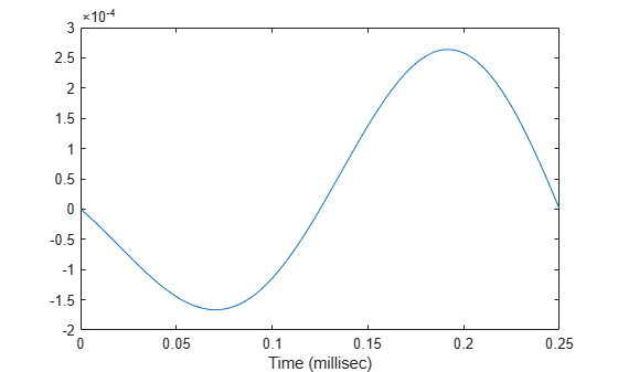

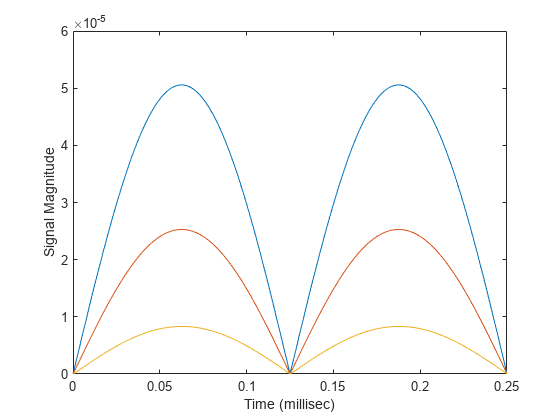
Propagate Signal to Multiple Destinations

Create a FreeSpace System object™ to propagate a signal from one point to multiple points in space. Start by defining a signal origin and three destination points, all at different ranges.

Compute the propagation direction angles from the source to the destination locations. The source and destination are stationary.

pos1 = [0,0,0]';
vel1 = [0,0,0]';
pos2 = [[700;700;100],[1400;1400;200],2*[2100;2100;400]];
vel2 = zeros(size(pos2));
[rngs,radiatingAngles] = rangeangle(pos2,pos1);

Create the cosine antenna element, ULA array, and Radiator System objects.

fs = 8000;
freq = 300e6;
nsensors = 4;
sAnt = phased.CosineAntennaElement;
sArray = phased.ULA('Element',sAnt,'NumElements',nsensors);
sRad = phased.Radiator('Sensor',sArray,...
    'OperatingFrequency',freq,...
    'CombineRadiatedSignals',true,'WeightsInputPort',true);

Create a signal to be one cycle of a sinusoid of amplitude one and having a frequency of 4 kHz.

fsig = 4000;
t = [0:0.01:2]'/fs;
signal = sin(2*pi*fsig*t);

Radiate the signals in the destination directions. Apply a uniform weighting to the array.

y = step(sRad,signal,radiatingAngles,[1,1,1,1].');

Propagate the signals to the destination points.

sFSp = phased.FreeSpace('OperatingFrequency',freq,'SampleRate',fs);
yprop = step(sFSp,y,pos1,pos2,vel1,vel2);

Plot the propagated signal magnitudes for each range.

figure
plot(1000*t,abs(yprop(:,1)),1000*t,abs(yprop(:,2)),1000*t,abs(yprop(:,3)))
ylabel('Signal Magnitude')
xlabel('Time (millisec)')

More About

Freespace Time Delay and Path Loss

When the origin and destination are stationary relative to each other, you can write the output signal of a free-space channel as Y(t) = x(t-τ)/L_fsp. The quantity τ is the signal delay and L_fsp is the free-space path loss. The delay τ is given by R/c, where R is the propagation distance and c is the propagation speed. The free-space path loss is given by

$$L_{fsp}=\frac{{(4\pi R)}^2}{{\lambda }^2},$$

where λ is the signal wavelength.

This formula assumes that the target is in the far field of the transmitting element or array. In the near field, the free-space path loss formula is not valid and can result in a loss smaller than one, equivalent to a signal gain. Therefore, the loss is set to unity for range values, R ≤ λ/4π.

When the origin and destination have relative motion, the processing also introduces a Doppler frequency shift. The frequency shift is v/λ for one-way propagation and 2v/λ for two-way propagation. The quantity v is the relative speed of the destination with respect to the origin.

For more details on free-space channel propagation, see [2].

References

[1] Proakis, J. Digital Communications. New York: McGraw-Hill, 2001.

[2] Skolnik, M. Introduction to Radar Systems, 3rd Ed. New York: McGraw-Hill, 2001.

Extended Capabilities

C/C++ Code Generation

Generate C and C++ code using MATLAB® Coder™.

Usage notes and limitations:

• Requires dynamic memory allocation. See Limitations for System Objects that Require Dynamic Memory Allocation.

• See System Objects in MATLAB Code Generation (MATLAB Coder).

Version History

Introduced in R2011a