Reduced-Order Modeling Technique for Beam with Point Load
This example shows how to eliminate degrees of freedom (DoFs) that are not on the boundaries of interest by using the Craig-Bampton reduced-order modeling technique. The example also uses the smaller dimension superelement to analyze the dynamics of the system. For comparison, the example also performs a direct transient analysis on the original structure.
Create a square cross-section beam geometry.
gm = multicuboid(0.05,0.003,0.003);
Plot the geometry, displaying face and edge labels.
pdegplot(gm,FaceLabels="on",FaceAlpha=0.3)
view([71 4])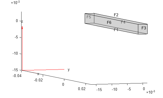
pdegplot(gm,EdgeLabels="on",FaceAlpha=0.3)
view([71 4])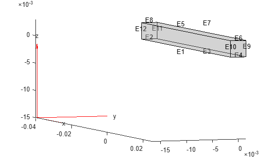
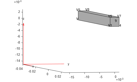
Add a vertex at the center of face 3.
loadedVertex = ...
    addVertex(gm,Coordinates=[0.025 0.0 0.0015]);
pdegplot(gm,VertexLabels="on")
view([78 2.5])
Create an femodel for transient structural analysis.
model = femodel(AnalysisType="structuralTransient", ...
                Geometry=gm);
Specify Young's modulus, Poisson's ratio, and the mass density of the material.
model.MaterialProperties = ...
    materialProperties(YoungsModulus=210E9, ...
                       PoissonsRatio=0.3, ...
                       MassDensity=7800);
Fix one end of the beam.
model.EdgeBC([2 8 11 12]) = edgeBC(Constraint="fixed");Generate a mesh.
model = generateMesh(model);
Define a sinusoidal load function, sinusoidalLoad, to model a harmonic load. This function accepts the load magnitude (amplitude), the location and state structure arrays, frequency, and phase. Because the function depends on time, it must return a matrix of NaN of the correct size when state.time is NaN. Solvers check whether a problem is nonlinear or time-dependent by passing NaN state values and looking for returned NaN values.
function Tn = sinusoidalLoad(load,location,state,Frequency,Phase)
if isnan(state.time)
    Tn = NaN*[location.nx location.ny location.nz];
    return
end
if isa(load,"function_handle")
    load = load(location,state);
else
    load = load(:);
end
Tn = load.*sin(Frequency.*state.time + Phase);
end
Apply a sinusoidal concentrated force in the z-direction on the new vertex.
Force=[0 0 10];
Frequency = 6000;
Phase = 0;
forcePulse = ...
    @(location,state) sinusoidalLoad(Force, ...
                                     location,state, ...
                                     Frequency,Phase);
model.VertexLoad(loadedVertex) = ...
    vertexLoad(Force=forcePulse);
Specify zero initial conditions.
model.CellIC = cellIC(Velocity=[0;0;0], ...
                      Displacement=[0;0;0]);
Solve the model.
tlist = 0:0.00005:3E-3;
RT = solve(model,tlist);
Specify the fixed and loaded boundaries as structural superelement interfaces by creating a romInterface object for each superelement interface. In this case, the reduced order model retains the degrees of freedom (DoFs) on the fixed face and the loaded vertex while condensing all other DoFs in favor of modal DoFs. For better performance, use the set of edges bounding face 5 instead of using the entire face.
romObj1 = romInterface(Edge=[2 8 11 12]);
romObj2 = romInterface(Vertex=loadedVertex);
Assign a vector of interface objects to the ROMInterfaces property of the model.
model.ROMInterfaces = [romObj1,romObj2];
Reduce the structure, retaining all fixed interface modes up to 5e5.
rom = reduce(model,FrequencyRange=[-0.1,5e5]);
Next, use the reduced order model to simulate the transient dynamics. Use the ode15s function directly to integrate the reduced system ODE. Working with the reduced model requires indexing into the reduced system matrices rom.K and rom.M. First, construct mappings of indices of K and M to loaded and fixed DoFs by using the data available in rom.
DoFs correspond to translational displacements. If the number of mesh points in a model is Nn, then the toolbox assigns the IDs to the DoFs as follows: the first 1 to Nn are x-displacements, Nn+1 to 2*Nn are y-displacements, and 2Nn+1 to 3*Nn are z-displacements. The reduced model object rom contains these IDs for the retained DoFs in rom.RetainedDoF.
Create a function that returns DoF IDs given node IDs and the number of nodes.
getDoF = @(x,numNodes) [x(:); x(:) + numNodes; x(:) + 2*numNodes];
Knowing the DoF IDs for the given node IDs, use the intersect function to find the required indices.
numNodes = size(rom.Mesh.Nodes,2);

loadedNode = findNodes(rom.Mesh,"region","Vertex",loadedVertex);
loadDoFs = getDoF(loadedNode,numNodes);
[~,loadNodeROMIds,~] = intersect(rom.RetainedDoF,loadDoFs);
In the reduced matrices rom.K and rom.M, generalized modal DoFs appear after the retained DoFs.
fixedIntModeIds = (numel(rom.RetainedDoF) + 1:size(rom.K,1))';
Because fixed-end DoFs are not a part of the ODE system, the indices for the ODE DoFs in reduced matrices are as follows.
odeDoFs = [loadNodeROMIds;fixedIntModeIds];
The relevant components of rom.K and rom.M for time integration are:
Kconstrained = rom.K(odeDoFs,odeDoFs);
Mconstrained = rom.M(odeDoFs,odeDoFs);
numODE = numel(odeDoFs);
Now you have a second-order system of ODEs. To use ode15s, convert this into a system of first-order ODEs by applying linearization. Such a first-order system is twice the size of the second-order system.
Mode = [eye(numODE,numODE),   zeros(numODE,numODE); ...
        zeros(numODE,numODE), Mconstrained];
Kode = [zeros(numODE,numODE), -eye(numODE,numODE); ...
        Kconstrained,         zeros(numODE,numODE)];
Fode = zeros(2*numODE,1);
The specified concentrated force load in the full system is along the z-direction, which is the third DoF in the ODE system. Accounting for the linearization to obtain the first-order system gives the loaded ODE DoF.
loadODEDoF = numODE + 3;
Specify the mass matrix and the Jacobian for the ODE solver.
odeoptions = odeset;
odeoptions = odeset(odeoptions,Jacobian=-Kode);
odeoptions = odeset(odeoptions,Mass=Mode);
Specify zero initial conditions.
u0 = zeros(2*numODE,1);
Solve the reduced system by using ode15s and the helper function CMSODEf.
function f = CMSODEf(t,u,Kode,Fode,loadedVertex)
Fode(loadedVertex) = 10*sin(6000*t);
f = -Kode*u +Fode;
end

sol = ode15s(@(t,y) CMSODEf(t,y,Kode,Fode,loadODEDoF), ...
                                 tlist,u0,odeoptions);
Compute the values of the ODE variable and the time derivatives.
[displ,vel] = deval(sol,tlist);
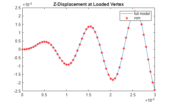
Plot the z-displacement at the loaded vertex and compare it to the third DoF in the solution of the reduced ODE system.
figure
plot(tlist,RT.Displacement.uz(loadedVertex,:))
hold on
plot(tlist,displ(3,:),"r*")
title("Z-Displacement at Loaded Vertex")
legend("full model","rom")
Knowing the solution in terms of the interface DoFs and modal DoFs, you can reconstruct the solution for the full model. The reconstructSolution function requires the displacement, velocity, and acceleration at all DoFs in rom. Construct the complete solution vector, including the zero values at the fixed DoFs.
u = zeros(size(rom.K,1),numel(tlist));
ut = zeros(size(rom.K,1),numel(tlist));
utt = zeros(size(rom.K,1),numel(tlist));
u(odeDoFs,:) = displ(1:numODE,:);
ut(odeDoFs,:) = vel(1:numODE,:);
utt(odeDoFs,:) = vel(numODE+1:2*numODE,:);
Construct a transient results object using this solution.
RTrom = reconstructSolution(rom,u,ut,utt,tlist);
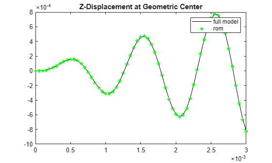
For comparison, compute the displacement in the interior at the center of the beam using the full and reconstructed solutions.
coordCenter = [0;0;0];
iDispRT = interpolateDisplacement(RT, coordCenter);
iDispRTrom = interpolateDisplacement(RTrom, coordCenter);
figure
plot(tlist,iDispRT.uz,"k")
hold on
plot(tlist,iDispRTrom.uz,"g*")
title("Z-Displacement at Geometric Center")
legend("full model","rom")