이 번역 페이지는 최신 내용을 담고 있지 않습니다. 최신 내용을 영문으로 보려면 여기를 클릭하십시오.

여러 문제 기반 접근법을 사용한 비선형 데이터 피팅

최소제곱 문제 설정에 대한 일반적인 지침은 문제가 최소제곱 형식임을 solve가 인식할 수 있는 방식으로 문제를 정식화하는 것입니다. 이렇게 하면 solve가 내부적으로 lsqnonlin을 호출하여 최소제곱 문제를 푸는 데 효율적이 됩니다. Write Objective Function for Problem-Based Least Squares 항목을 참조하십시오.

이 예제에서는 동일한 문제에서 lsqnonlin의 성능과 fminunc의 성능을 비교하여 최소제곱 솔버의 효율성을 보여줍니다. 또한, 문제의 선형 부분을 명시적으로 인식하고 별도로 처리하여 얻을 수 있는 추가적인 이점도 보여줍니다.

문제 설정

다음과 같은 데이터가 있다고 가정하겠습니다.

Data = ...
  [0.0000    5.8955
   0.1000    3.5639
   0.2000    2.5173
   0.3000    1.9790
   0.4000    1.8990
   0.5000    1.3938
   0.6000    1.1359
   0.7000    1.0096
   0.8000    1.0343
   0.9000    0.8435
   1.0000    0.6856
   1.1000    0.6100
   1.2000    0.5392
   1.3000    0.3946
   1.4000    0.3903
   1.5000    0.5474
   1.6000    0.3459
   1.7000    0.1370
   1.8000    0.2211
   1.9000    0.1704
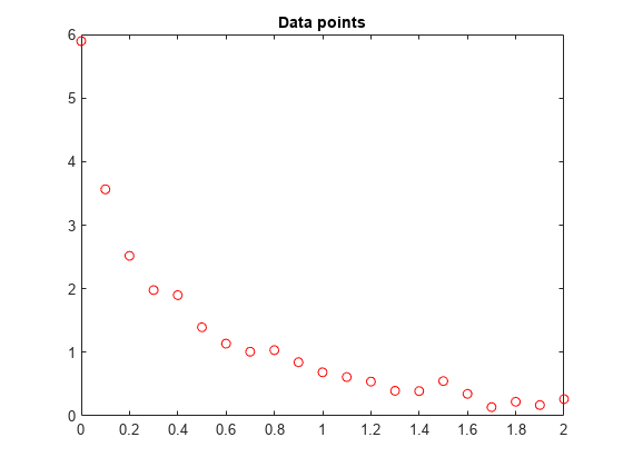
   2.0000    0.2636];

데이터 점을 플로팅합니다.

t = Data(:,1);
y = Data(:,2);
plot(t,y,'ro')
title('Data points')

다음 함수를 피팅하는 문제입니다.

y = c(1)*exp(-lam(1)*t) + c(2)*exp(-lam(2)*t)

데이터에 피팅해 보겠습니다.

디폴트 솔버를 사용하는 풀이법

먼저, 방정식에 대응하는 최적화 변수를 정의합니다.

c = optimvar('c',2);
lam = optimvar('lam',2);

초기점 x0을 c(1) = 1, c(2) = 1, lam(1) = 1, lam(2) = 0과 같이 임의로 설정합니다.

x0.c = [1,1];
x0.lam = [1,0];

파라미터가 c 및 lam인 경우 시간 t에서의 응답 값을 계산하는 함수를 만듭니다.

diffun = c(1)*exp(-lam(1)*t) + c(2)*exp(-lam(2)*t);

diffun을 이 함수와 데이터 y 사이 차의 제곱합을 계산하는 최적화 표현식으로 변환합니다.

diffexpr = sum((diffun - y).^2);

diffexpr을 목적 함수로 갖는 최적화 문제를 만듭니다.

ssqprob = optimproblem('Objective',diffexpr);

디폴트 솔버를 사용하여 문제를 풉니다.

[sol,fval,exitflag,output] = solve(ssqprob,x0)

Solving problem using lsqnonlin.

Local minimum possible.

lsqnonlin stopped because the final change in the sum of squares relative to 
its initial value is less than the value of the function tolerance.

sol = struct with fields:
      c: [2x1 double]
    lam: [2x1 double]

fval = 0.1477

exitflag = 
    FunctionChangeBelowTolerance

output = struct with fields:
           firstorderopt: 7.8870e-06
              iterations: 6
               funcCount: 7
            cgiterations: 0
               algorithm: 'trust-region-reflective'
                stepsize: 0.0096
                 message: 'Local minimum possible....'
            bestfeasible: []
         constrviolation: []
     objectivederivative: "forward-AD"
    constraintderivative: "closed-form"
                  solver: 'lsqnonlin'

반환된 해 값 sol.c와 sol.lam을 기반으로 하여 결과 곡선을 플로팅합니다.

resp = evaluate(diffun,sol);
hold on
plot(t,resp)
hold off

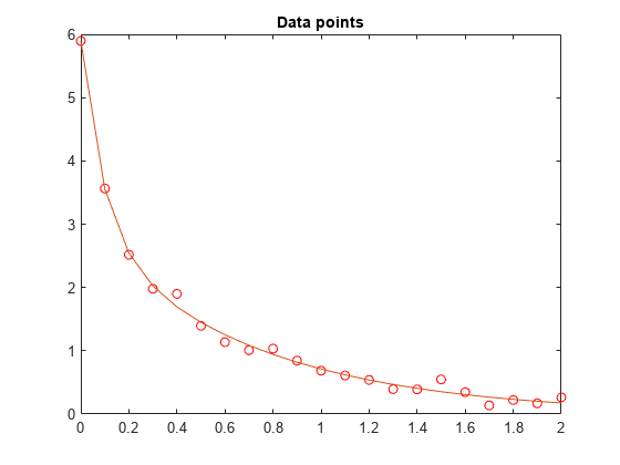
피팅이 가능한 잘 맞는 것처럼 보입니다.

fminunc를 사용하는 풀이법

fminunc 솔버를 사용하여 문제를 풀려면 solve를 호출할 때 'Solver' 옵션을 'fminunc'로 설정하십시오.

[xunc,fvalunc,exitflagunc,outputunc] = solve(ssqprob,x0,'Solver',"fminunc")

Solving problem using fminunc.

Local minimum found.

Optimization completed because the size of the gradient is less than
the value of the optimality tolerance.

xunc = struct with fields:
      c: [2x1 double]
    lam: [2x1 double]

fvalunc = 0.1477

exitflagunc = 
    OptimalSolution

outputunc = struct with fields:
             iterations: 30
              funcCount: 37
               stepsize: 0.0017
           lssteplength: 1
          firstorderopt: 2.9454e-05
              algorithm: 'quasi-newton'
                message: 'Local minimum found....'
    objectivederivative: "forward-AD"
                 solver: 'fminunc'

fminunc는 lsqcurvefit과 동일한 해를 구했지만 함수 실행 횟수가 훨씬 많았음을 알 수 있습니다. fminunc의 파라미터는 lsqcurvefit의 파라미터와 순서가 반대입니다. 즉, lam(1)이 아니라 lam(2)가 더 큰 lam입니다. 변수의 순서는 임의로 지정 가능하므로 이는 놀랍지 않은 일입니다.

fprintf(['There were %d iterations using fminunc,' ...
    ' and %d using lsqcurvefit.\n'], ...
    outputunc.iterations,output.iterations)

There were 30 iterations using fminunc, and 6 using lsqcurvefit.

fprintf(['There were %d function evaluations using fminunc,' ...
    ' and %d using lsqcurvefit.'], ...
    outputunc.funcCount,output.funcCount)

There were 37 function evaluations using fminunc, and 7 using lsqcurvefit.

선형 문제와 비선형 문제로 분리하기

이 피팅 문제는 파라미터 c(1)과 c(2)에서 선형 문제임을 알 수 있습니다. 이는 lam(1)과 lam(2)의 모든 값에 대해 백슬래시 연산자를 사용하여 c(1)과 c(2)의 값을 구하여 최소제곱 문제를 풀 수 있음을 의미합니다.

이 문제를 2차원 문제로 다시 구성하여 lam(1)과 lam(2)에 대한 최적의 값을 찾아보겠습니다. c(1)과 c(2)의 값은 위에 설명한 대로 각 단계에서 백슬래시 연산자를 사용하여 계산됩니다. 이를 위해, 매 솔버 반복에서 c(1)과 c(2)를 얻기 위해 백슬래시 연산을 수행하는 fitvector 함수를 사용합니다.

type fitvector

function yEst = fitvector(lam,xdata,ydata)
%FITVECTOR  Used by DATDEMO to return value of fitting function.
%   yEst = FITVECTOR(lam,xdata) returns the value of the fitting function, y
%   (defined below), at the data points xdata with parameters set to lam.
%   yEst is returned as a N-by-1 column vector, where N is the number of
%   data points.
%
%   FITVECTOR assumes the fitting function, y, takes the form
%
%     y =  c(1)*exp(-lam(1)*t) + ... + c(n)*exp(-lam(n)*t)
%
%   with n linear parameters c, and n nonlinear parameters lam.
%
%   To solve for the linear parameters c, we build a matrix A
%   where the j-th column of A is exp(-lam(j)*xdata) (xdata is a vector).
%   Then we solve A*c = ydata for the linear least-squares solution c,
%   where ydata is the observed values of y.

A = zeros(length(xdata),length(lam));  % build A matrix
for j = 1:length(lam)
   A(:,j) = exp(-lam(j)*xdata);
end
c = A\ydata; % solve A*c = y for linear parameters c
yEst = A*c; % return the estimated response based on c

solve를 사용하여 2차원 초기점 x02.lam = [1,0]부터 시작해 문제를 풉니다. 이를 위해, 먼저 fcn2optimexpr을 사용하여 fitvector 함수를 최적화 표현식으로 변환합니다. Convert Nonlinear Function to Optimization Expression 항목을 참조하십시오. 경고가 발생하지 않도록 하기 위해 결과 표현식의 출력 크기를 지정합니다. 변환된 fitvector 함수와 데이터 y 사이 차의 제곱합을 목적 함수로 가지는 새 최적화 문제를 만듭니다.

x02.lam = x0.lam;
F2 = fcn2optimexpr(@(x) fitvector(x,t,y),lam,'OutputSize',[length(t),1]);
ssqprob2 = optimproblem('Objective',sum((F2 - y).^2));
[sol2,fval2,exitflag2,output2] = solve(ssqprob2,x02)

Solving problem using lsqnonlin.

Local minimum possible.

lsqnonlin stopped because the final change in the sum of squares relative to 
its initial value is less than the value of the function tolerance.

sol2 = struct with fields:
    lam: [2x1 double]

fval2 = 0.1477

exitflag2 = 
    FunctionChangeBelowTolerance

output2 = struct with fields:
           firstorderopt: 4.4087e-06
              iterations: 10
               funcCount: 33
            cgiterations: 0
               algorithm: 'trust-region-reflective'
                stepsize: 0.0080
                 message: 'Local minimum possible....'
            bestfeasible: []
         constrviolation: []
     objectivederivative: "finite-differences"
    constraintderivative: "closed-form"
                  solver: 'lsqnonlin'

2차원 풀이법과 4차원 풀이법의 효율성은 서로 비슷합니다.

fprintf(['There were %d function evaluations using the 2-d ' ...
    'formulation, and %d using the 4-d formulation.'], ...
    output2.funcCount,output.funcCount)

There were 33 function evaluations using the 2-d formulation, and 7 using the 4-d formulation.

분리된 문제가 초기 추측값에 대해 더 견고함

4개의 파라미터를 갖는 원래 문제에서 잘못된 시작점을 선택하면 전역해가 아닌 국소해를 찾습니다. 2개의 파라미터로 분리된 문제에서 똑같이 잘못된 lam(1) 값과 lam(2) 값을 갖는 시작점을 선택하는 경우에는 전역해를 찾습니다. 이를 확인하기 위해 상대적으로 나쁜 국소해를 생성하게 하는 시작점을 사용하여 원래 문제를 다시 실행한 후 결과로 생성되는 피팅을 전역해와 비교해 보겠습니다.

x0bad.c = [5 1];
x0bad.lam = [1 0];
[solbad,fvalbad,exitflagbad,outputbad] = solve(ssqprob,x0bad)

Solving problem using lsqnonlin.

Local minimum possible.

lsqnonlin stopped because the final change in the sum of squares relative to 
its initial value is less than the value of the function tolerance.

solbad = struct with fields:
      c: [2x1 double]
    lam: [2x1 double]

fvalbad = 2.2173

exitflagbad = 
    FunctionChangeBelowTolerance

outputbad = struct with fields:
           firstorderopt: 0.0036
              iterations: 31
               funcCount: 32
            cgiterations: 0
               algorithm: 'trust-region-reflective'
                stepsize: 0.0012
                 message: 'Local minimum possible....'
            bestfeasible: []
         constrviolation: []
     objectivederivative: "forward-AD"
    constraintderivative: "closed-form"
                  solver: 'lsqnonlin'

respbad = evaluate(diffun,solbad);
hold on
plot(t,respbad,'g')
legend('Data','Global fit','Bad local fit','Location','NE')
hold off

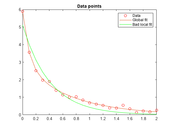
fprintf(['The residual norm at the good ending point is %f,' ...
   ' and the residual norm at the bad ending point is %f.'], ...
   fval,fvalbad)

The residual norm at the good ending point is 0.147723, and the residual norm at the bad ending point is 2.217300.

참고 항목

solve | fcn2optimexpr

관련 항목

• 비선형 데이터 피팅
• 문제 기반 최적화 워크플로