Generate and Plot Pareto Front
This example shows how to generate and plot a Pareto front for a 2-D multiobjective function using fgoalattain.
The two objective functions in this example are shifted and scaled versions of the convex function . The code for the objective functions appears in the simple_mult helper function at the end of this example.
Both objective functions decrease in the region and increase in the region . In between 0 and 1, increases and decreases, so a tradeoff region exists. Plot the two objective functions for ranging from to .
t = linspace(-1/2,3/2);
F = simple_mult(t);
plot(t,F,LineWidth=2)
hold on
plot([0,0],[0,8],"g--");
plot([1,1],[0,8],"g--");
plot([0,1],[1,6],"k.",MarkerSize=15);
text(-0.25,1.5,"Minimum(f_1(x))")
text(.75,5.5,"Minimum(f_2(x))")
hold off
legend("f_1(x)","f_2(x)")
xlabel({"x";"Tradeoff region between the green lines"})
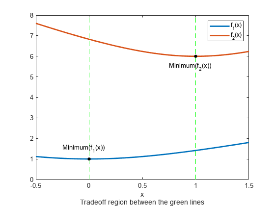
To find the Pareto front, first find the unconstrained minima of the two objective functions. In this case, you can see in the plot that the minimum of is 1, and the minimum of is 6, but in general you might need to use an optimization routine to find the minima.
In general, write a function that returns a particular component of the multiobjective function. (The pickindex helper function at the end of this example returns the th objective function value.) Then find the minimum of each component using an optimization solver. You can use fminbnd in this case, or fminunc for higher-dimensional problems.
k = 1;
[min1,minfn1] = fminbnd(@(x)pickindex(x,k),-1,2);
k = 2;
[min2,minfn2] = fminbnd(@(x)pickindex(x,k),-1,2);
Set goals that are the unconstrained optima for each objective function. You can simultaneously achieve these goals only if the objective functions do not interfere with each other, meaning there is no tradeoff.
goal = [minfn1,minfn2];
To calculate the Pareto front, take weight vectors for from 0 through 1. Solve the goal attainment problem, setting the weights to the various values.
nf = 2; % Number of objective functions
N = 50; % Number of points for plotting
onen = 1/N;
x = zeros(N+1,1);
f = zeros(N+1,nf);
fun = @simple_mult;
x0 = 0.5;
options = optimoptions("fgoalattain",Display="off");
for r = 0:N
t = onen*r; % 0 through 1
weight = [t,1-t];
[x(r+1,:),f(r+1,:)] = fgoalattain(fun,x0,goal,weight,...
[],[],[],[],[],[],[],options);
end
figure
plot(f(:,1),f(:,2),"ko");
xlabel("f_1")
ylabel("f_2")
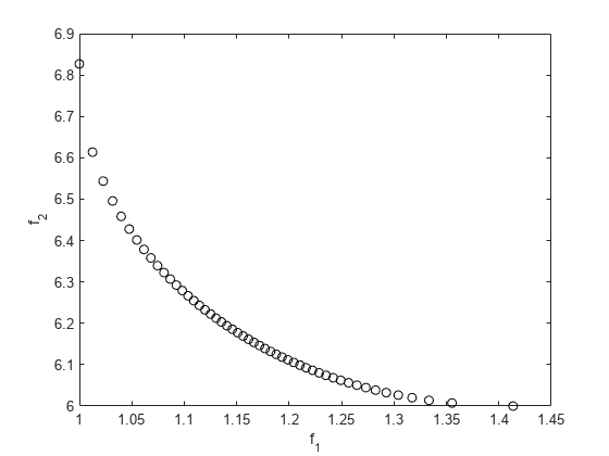
You can see the tradeoff between the two objective functions.
Helper Functions
The following code creates the simple_multi function.
function f = simple_mult(x)
f(:,1) = sqrt(1+x.^2);
f(:,2) = 4 + 2*sqrt(1+(x-1).^2);
end
The following code creates the pickindex function.
function z = pickindex(x,k)
z = simple_mult(x); % evaluate both objectives
z = z(k); % return objective k
end