Adjust Input and Output Weights Based on Sensitivity Analysis
This example shows how to compute numerical derivatives of a cumulative performance index with respect to the weights of the MPC quadratic cost function, and use these derivatives to improve performance.
Define Plant Model
Create a state-space model for the plant.
plant = ss(tf( ...
    {1,1,2;1 -1 -1}, ...
    {[1 0 0],[1 0 0],[1 1];[1 2 8],[1 3],[1 1 3]}), ...
    'min');
The model is continuous-time and has 3 inputs (assumed to be manipulated variables), 2 outputs (assumed to be both measurable), and 8 state variables.
Design MPC Controller
Create an MPC controller with a sample time of 0.1, a prediction horizon of 20 steps, and a control horizon of 3 steps.
mpcobj = mpc(plant,0.1,20,3);
-->"Weights.ManipulatedVariables" is empty. Assuming default 0.00000.
-->"Weights.ManipulatedVariablesRate" is empty. Assuming default 0.10000.
-->"Weights.OutputVariables" is empty. Assuming default 1.00000.
Set constraints on manipulated variables and their rates of change.
for i = 1:3
    mpcobj.MV(i).Min = -2;
    mpcobj.MV(i).Max = 2;
    mpcobj.MV(i).RateMin = -4;
    mpcobj.MV(i).RateMax = 4;
end
Display the default cost function weights for the output variables, manipulated variables and manipulated variables rate.
mpcobj.Weights.OutputVariables
ans = 1×2

     1     1
mpcobj.Weights.ManipulatedVariables
ans = 1×3

     0     0     0
mpcobj.Weights.ManipulatedVariablesRate
ans = 1×3

    0.1000    0.1000    0.1000
Performance Evaluation Setup
Define a closed-loop cumulative performance index as the weighted Integral of the Square Error (ISE) between the plant signals and their references, calculated in the interval from 0 to Tstop seconds.
The weights, which reflect the desired closed-loop behavior, must be contained in a structure with the same fields as the Weights property of an MPC object.
perfWeights = mpcobj.weights;
In this example, output tracking is more important than keeping the manipulated variable values low, therefore, define relatively higher weights on the output error, slightly higher weights on the manipulated variable rate, and keep the default weights on the manipulated variable values.
perfWeights.OutputVariables = [100 100];
perfWeights.ManipulatedVariablesRate = [1 1 1];
Note that perfWeights is used only to calculate the cumulative performance index. It is not related to the weights specified inside the MPC controller object. Therefore the cumulative performance index is not related to the quadratic cost function that the MPC controller tries to minimize by choosing the manipulated variable values. Indeed, the performance index is based on a closed loop simulation until a time that is generally different than the prediction horizon, while the MPC controller calculates the moves which minimize its internal cost function up to the prediction horizon and in open loop fashion. Furthermore, even when the performance index is chosen to be of ISE type, its weights should be squared to match the weights defined in the MPC cost function.
Setup Simulation Parameters and Signals
In this example, you calculate the cumulative performance index sensitivity within a setpoint tracking scenario.
Tstop = 80;              % number of time steps to be simulated
r = ones(Tstop,1)*[1 1]; % set point reference signals
v = [];                  % no disturbance is added
sopts = mpcsimopt;      % create simulation options object
sopts.PlantInitialState = zeros(8,1); % set plant initial state
Calculate Sensitivities
Calculate the performance index value and its sensitivities to the mpcobj cost function weights, using the sensitivity function.
[J1, Sens1] = sensitivity(mpcobj,'ISE',perfWeights,Tstop,r,v,sopts);-->Converting model to discrete time. Assuming no disturbance added to measured output #1. -->Integrator added as output disturbance model for measured output #2. -->"Model.Noise" is empty. Assuming white noise on each measured output.
Display sensitivities with respect to the weights for the output error signals, .
Sens1.OutputVariables
ans = 1×2
104 ×
-2.7346 2.7166
Display sensitivities with respect to the weights for the manipulated variable signals, .
Sens1.ManipulatedVariables
ans = 1×3
3.3375 -125.8266 -35.1067
Display sensitivities with respect to the weights for the manipulated variables rate signals, .
Sens1.ManipulatedVariablesRate
ans = 1×3
104 ×
-0.0007 1.0250 -0.8370
Adjust MPC Weights
Since you want to reduce the closed-loop cumulative performance index J, in this example the derivatives with respect to output weights show that the weight on y1 should be increased, as the corresponding derivative is negative, while the weight on y2 should be decreased.
Copy the MPC object to make modification on the new object.
mpcobj_new = mpcobj;
A negative sensitivity suggests increasing the first output weight from 1 to 2.
mpcobj_new.Weights.OutputVariables(1) = 2;
A positive sensitivity suggests decreasing the second output weight from 1 to 0.2.
mpcobj_new.Weights.OutputVariables(2) = 0.2;
Note that the sensitivity analysis only tells you in which direction to change the parameters, but not by how much. A trial and error procedure to select the appropriate magnitude of the change is expected.
Verify Performance Changes
Simulate both MPC controllers.
[y1, t1, u1] = sim(mpcobj, Tstop, r, v, sopts); [y2, t2, u2] = sim(mpcobj_new, Tstop, r, v, sopts);
-->Converting model to discrete time.
   Assuming no disturbance added to measured output #1.
-->Integrator added as output disturbance model for measured output #2.
-->"Model.Noise" is empty. Assuming white noise on each measured output.
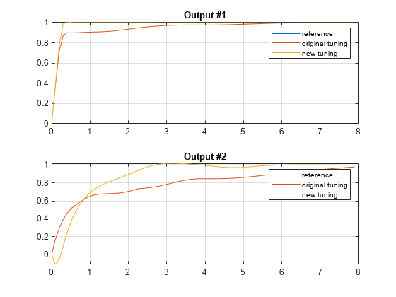
Plot simulation results for both controllers.
% Plot plant outputs
h1 = figure;

subplot(211)
plot(t2,r(:,1),t1,y1(:,1),t2,y2(:,1));grid
legend('reference','original tuning','new tuning')
title('Output #1')

subplot(212)
plot(t2,r(:,2),t1,y1(:,2),t2,y2(:,2));grid
legend('reference','original tuning','new tuning')
title('Output #2')
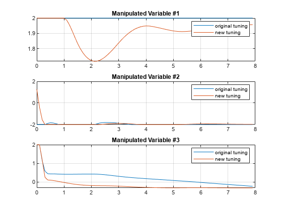
% Plot manipulated variables
h2 = figure;

subplot(311)
plot(t1,u1(:,1),t2,u2(:,1));grid
legend('original tuning','new tuning')
title('Manipulated Variable #1')

subplot(312)
plot(t1,u1(:,2),t2,u2(:,2));grid
legend('original tuning','new tuning')
title('Manipulated Variable #2')

subplot(313)
plot(t1,u1(:,3),t2,u2(:,3));grid
legend('original tuning','new tuning')
title('Manipulated Variable #3')
Verify Cumulative Performance Index Is Reduced
Compute the cumulative performance index for the new controller using the same performance measure.
J2 = sensitivity(mpcobj_new,'ISE',perfWeights,Tstop,r,v,sopts);-->Converting model to discrete time. Assuming no disturbance added to measured output #1. -->Integrator added as output disturbance model for measured output #2. -->"Model.Noise" is empty. Assuming white noise on each measured output.
Previous Cumulative Performance Index.
J1
J1 =
1.2865e+05
New Cumulative Performance Index.
J2
J2 =
1.1623e+05
As expected the new value of the cumulative performance index is lower than the old value.
Use a User-Defined Performance Function
This is an example of how to write a user-defined performance function used by the sensitivity method. In this example, the custom function custom_performance_function.m implements the standard ISE performance index based on PerformanceWeights.
Display the function.
type custom_performance_function.mfunction J = custom_performance_function(mpcobj, perfWeights, Tsteps, r) % This is an example of how to write a user defined performance function % used by the "sensitivity" method. In this example, the code illustrates % using performance weights to compute the cumulative performance index. % Copyright 1990-2014 The MathWorks, Inc. % Carry out simulation [y,t,u] = sim(mpcobj, Tsteps, r); du = [u(1,:);diff(u)]; % Get Weights in mpcobj ny = size(mpcobj,'mo') + size(mpcobj,'uo'); nmv = size(mpcobj,'mv'); Wy = perfWeights.OutputVariables(:);Wy=Wy(1:ny); Wu = perfWeights.ManipulatedVariables(:);Wu=Wu(1:nmv); Wdu = perfWeights.ManipulatedVariablesRate(:);Wdu=Wdu(1:nmv); % Set mv target to 0 utarget=zeros(nmv,1); % Compute J in ISE form J=0; aux=(y-r)*Wy; J=J+aux'*aux; aux=(u-ones(Tsteps,1)*utarget')*Wu; J=J+aux'*aux; aux=du*Wdu; J=J+aux'*aux;
Use the custom function to calculate the performance index.
J3 = sensitivity(mpcobj,'custom_performance_function', ...
    perfWeights,Tstop,r)
J3 =
1.2865e+05
As expected, for mpcobj, user-defined Cumulative Performance Index J3 has the same value as J1.