Overmodulation
R2026bExtend voltage utilization beyond the linear modulation region using single-zone overmodulation
Since R2026b
Overmodulation block
To add a block to a model, double-click the canvas and start typing the block name. Then, select the block from the list.
Libraries:
Motor Control Blockset /
Math Transforms
Description
The Overmodulation block enables the application of reference voltages beyond the space vector pulse width modulation (SVPWM) linear modulation limit using a single-zone overmodulation algorithm. Use this block if your motor application requires speeds above base speed or higher torque output than what linear SVPWM can provide. Place this block between the output of the current controller (or inverse Park transform) and the SVPWM generator in the field-oriented control (FOC) control loop.
The block automatically detects and operates in three regions based on reference voltage magnitude:
Linear region — The reference magnitude is at or below . The block passes the reference through without change.
Overmodulation region — The reference magnitude exceeds but is below . The block modifies both the magnitude and angle of the output voltage vector, clamping it to the inverter hexagonal boundary.
Six-step region — The reference magnitude exceeds . The block drives the output to the hexagon vertices, producing six-step commutation waveforms.
Note
The block does not implement hysteresis for region transitions. If the reference voltage magnitude is slightly above a threshold, the block immediately enters the higher region. For example, a reference magnitude marginally above places the block in the six-step region.
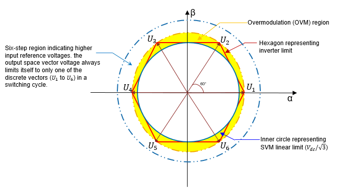
By transitioning through these three regions, the fundamental voltage component increases from (linear limit) to (six-step limit), representing approximately a 10% gain over conventional linear SVPWM. This extended voltage range allows your motor to achieve higher speeds and produce more torque without requiring a higher DC bus voltage.
Unlike traditional discrete mode-switching approaches, this block implements a unified voltage conversion strategy that operates continuously across all three regions without mode switching. Beyond the linear limit, the block converts the input voltage reference into an output that increasingly resembles a square wave as it approaches six-step commutation, allowing the FOC system to apply the maximum available fundamental voltage to the motor without discontinuities at region transitions.
Set the Voltage input type parameter to match your upstream
controller output. Select Alpha and beta to provide alpha-beta
voltage components directly from the current controller or inverse Park transform, or
select Magnitude and position to provide the voltage magnitude and
electrical position as separate signals. Monitor the Info output
bus to track transitions across all three operating regions through the
ModulationState signal.
Examples
This example shows how to use the Overmodulation block to extend inverter voltage utilization beyond the linear space vector pulse-width modulation (SVPWM) limit. This example uses a minimal model that drives the block with a linearly increasing alpha-axis voltage reference, which causes the operating region to sweep from linear modulation through the overmodulation region and into six-step commutation.
Using this example, you can observe the automatic transition from linear modulation to overmodulation to six-step commutation using the ModulationState signal and verify that the output voltage magnitude is clamped to the inverter hexagon boundary rather than growing unbounded.
Model
To focus on the Overmodulation block behavior, the example uses a model that feeds it a linearly increasing alpha-beta voltage reference. The value of 100 V sets the hexagon boundary thresholds. The block enters the overmodulation region when the reference magnitude exceeds V, and enters the six-step region when it exceeds V. A ramp starting at 20 V with slope 70 V/s sweeps through all three regions. Setting Vbeta to zero keeps the voltage vector on the alpha axis, which is the simplest input that covers all regions.
Open the model.
mdl = "OvermodulationRegions";
open_system(mdl)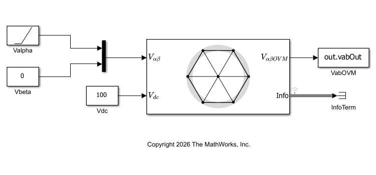
Simulate and Inspect Regions
To observe how the block responds across all three regions, simulate the model and extract the ModulationState and VMagOVM signals from the logged Info bus. ModulationState identifies the current region (0 = linear, 1 = overmodulation, 2 = six-step). VMagOVM is the magnitude of the modified output voltage vector. In the linear region it tracks the input, and in the overmodulation and six-step regions it is clamped to the hexagon boundary.
out = sim(mdl);
info = out.logsout{1}.Values
info = struct with fields:
VMagOVM: [1×1 timeseries]
ThetaOVM: [1×1 timeseries]
ModulationState: [1×1 timeseries]
HoldingAngle: [1×1 timeseries]
Analyze Modulation State Transition
To verify the transition through all three regions and see how the output vector is constrained geometrically, plot ModulationState versus time alongside the space vector trajectory in the αβ plane. In the αβ plot, the hexagon boundary (black) is the maximum voltage the inverter can produce at each angle. The inscribed circle (blue dashed, radius V) is the linear region limit, and the circumscribed circle (red dashed, radius V) is the six-step threshold. The green trajectory sweeps along the positive α-axis because Vbeta is zero: it grows freely in the linear region, is clamped to the hexagon edge in the overmodulation region, and terminates at the hexagon vertex in the six-step region.
Vdc = 100;
modState = info.ModulationState.Data;
t = info.VMagOVM.Time;
theta = linspace(0, 2*pi, 500);
hex_v = (2*Vdc/3) * exp(1i * (0:5)*pi/3);
hex_x = [real(hex_v), real(hex_v(1))];
hex_y = [imag(hex_v), imag(hex_v(1))];
Va = out.vabOut.Data(1:10:end, 1);
Vb = out.vabOut.Data(1:10:end, 2);

figure('Position',[100 100 900 380]);
tiledlayout(1,2,'TileSpacing','compact','Padding','compact');

nexttile;
plot(t, modState);
yticks([0 1 2]);
yticklabels(["Linear", "Overmodulation", "Six-Step"]);
ylabel('Region');
xlabel('Time (s)');
title('Modulation State vs. Time');
grid on;

nexttile;
hold on;
plot(hex_x, hex_y, 'k-', 'LineWidth', 1.5);
plot((Vdc/sqrt(3))*cos(theta), (Vdc/sqrt(3))*sin(theta), 'b--');
plot((2*Vdc/3)*cos(theta), (2*Vdc/3)*sin(theta), 'r--');
plot(Va, Vb, 'Color', [0.2 0.6 0.2], 'LineWidth', 2);
hold off;
grid on;
xlim([-80 80]); ylim([-80 80]);
xlabel('\alpha'); ylabel('\beta');
title('Space Vector Trajectory');
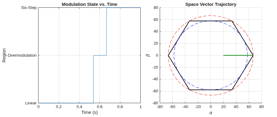
The modulation state plot confirms the block transitions from linear to overmodulation at approximately 0.54 s, and from overmodulation to six-step at approximately 0.67 s. The αβ plot shows the same behavior geometrically. The output trajectory (green) follows the reference exactly inside the inscribed circle, is constrained to the hexagon edge in the overmodulation region, and terminates at the hexagon vertex in the six-step region.
Extended Examples
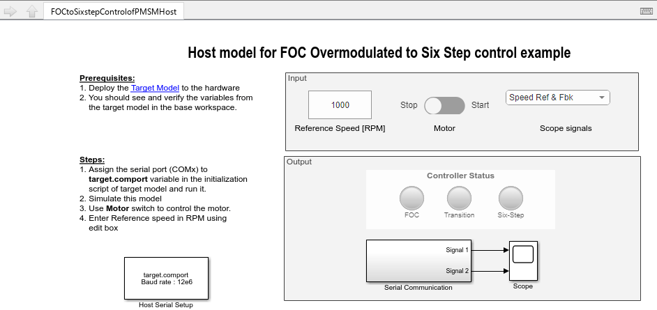
Field-oriented Control of PMSM with Six-Step Transition
Implement dynamic overmodulation to control a surface-mount permanent magnet synchronous motor (SPMSM) using field-oriented control (FOC). When the motor needs to reach higher speeds or produce more torque, the control method seamlessly transitions to six-step control. This allows the motor application to achieve better range without increasing the DC bus voltage of the inverter.
Ports
Input
Output
Parameters
References
[1] Bolognani, Silverio, and Mauro Zigliotto. "Novel Digital Continuous Control of SVM Inverters in the Overmodulation Range." IEEE Transactions on Industry Applications 33, no. 2 (March/April 1997): 525–530.
Extended Capabilities
Version History
Introduced in R2026b

