geoplot3
Geographic globe plot
Description
geoplot3(___, specifies
additional options for the line using one or more name-value arguments. Specify the options
after all other input arguments. For a list of options, see Line Properties.Name=Value)
p = geoplot3(___) returns a Line
object. This syntax is useful for controlling the properties of the line.
Examples
Plot the path of a glider above a local region. First, import sample data representing the path. Get the latitude, longitude, and geoid height values.
trk = readgeotable("sample_mixed.gpx",Layer="track_points");
lat = trk.Shape.Latitude;
lon = trk.Shape.Longitude;
h = trk.Elevation;
Create a geographic globe. Then, plot the path as a line.
uif = uifigure;
g = geoglobe(uif);
geoplot3(g,lat,lon,h,"c")
By default, the view is directly above the data. Change the view by setting the camera position, pitch angle, and heading angle.
campos(g,44.44,-72.81,9e3)
campitch(g,-30)
camheading(g,40)

When you plot a line between points that are far apart, the data may be obscured because the line passes through the Earth. View the entire line by inserting points between the specified data points.
For example, specify the coordinates of New York City and Paris. Then, plot a line between them. Indicate there is no height data by specifying the fourth argument of geoplot3 as an empty array. Note that you cannot see the line because it passes through the Earth.
lat = [40.71 48.86];
lon = [-74.01 2.35];
uif = uifigure;
g = geoglobe(uif);
geoplot3(g,lat,lon,[],"y",LineWidth=2)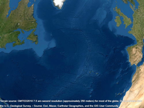
To see the line, insert points along a great circle using the interpm function. Then, plot the line again. Note that the line is visible.
[latI,lonI] = interpm(lat,lon,0.1,"gc");
geoplot3(g,latI,lonI,[],"y",LineWidth=2)

When you plot a line over a large region such as a state or country, part of the line may be obscured because it passes through terrain. View the entire line by removing the terrain data from the globe.
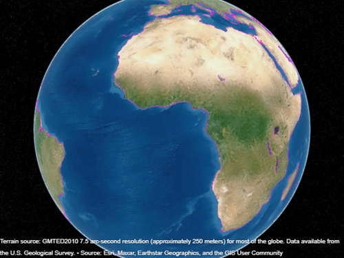
For example, import sample coastline data and plot it on a geographic globe. By default, the globe includes terrain data derived from the GMTED2010 model. Note that the line appears broken.
load coastlines
uif = uifigure;
g = geoglobe(uif);
p = geoplot3(g,coastlat,coastlon,[],"m");
To see the line, set the Terrain property of the globe to "none". Indicate the plotted data sits on the WGS84 reference ellipsoid by setting the HeightReference property of the line to "ellipsoid". Note that the line is visible over the basemap.
g.Terrain = "none";
p.HeightReference = "ellipsoid";
Import sample data representing the path of a glider. Get the latitude, longitude, and geoid height values.
trk = readgeotable("sample_mixed.gpx",Layer="track_points");
lat = trk.Shape.Latitude;
lon = trk.Shape.Longitude;
h = trk.Elevation;
Create a geographic globe. Then, plot the data using circle markers. Plot a marker at every 25th data point by setting the MarkerIndices property.
uif = uifigure;
g = geoglobe(uif);
mskip = 1:25:length(lat);
geoplot3(g,lat,lon,h,"mo",MarkerIndices=mskip)
Plot a line from the surface of Gross Reservoir to a point above South Boulder Peak.
Specify the latitude, longitude, and height of the two endpoints. Specify the heights relative to the terrain, so that 0 represents ground level and not sea level.
lat = [39.95384 39.95];
lon = [-105.29916 -105.3608];
hTerrain = [10 0];
Plot the line on a geographic globe. Indicate that height values are referenced to the terrain using the HeightReference property. By default, the view is directly above the data. Tilt the view by holding Ctrl and dragging.
uif = uifigure;
g = geoglobe(uif);
geoplot3(g,lat,lon,hTerrain,"y",HeightReference="terrain",LineWidth=3)

In many cases, the camera view of the geographic globe changes when you plot new data. You can preserve the camera view by setting the camera modes to "manual" and the hold state to "on".
Read the buildings layer from an OpenStreetMap file [1] containing data for several city blocks in Shibuya, Tokyo, Japan. Display the buildings in a geographic globe with a road map and no terrain data.
GT = readgeotable("shibuya.osm",Layer="buildings");
addCustomBuildings("shibuya",GT)

uif = uifigure;
g = geoglobe(uif,Buildings="shibuya",Basemap="streets-light",Terrain="none");
Adjust the camera view by interacting with the globe.
Read track points from a GPX file into a geospatial table. Extract the latitude and longitude coordinates from the geospatial table, and specify a height value for each coordinate.
track = readgeotable("shibuya_track.gpx",Layer="track_points");
lat = track.Shape.Latitude;
lon = track.Shape.Longitude;
height = linspace(10,100,length(lat));
Set the camera modes to "manual" and the hold state to "on". Then, plot the data. Note that the camera position does not change.
campos(g,"manual")
camheight(g,"manual")
camheading(g,"manual")
campitch(g,"manual")
camroll(g,"manual")
hold(g,"on")

geoplot3(g,lat,lon,height,"-o",LineWidth=3)
[1] You can download OpenStreetMap files from https://www.openstreetmap.org, which provides access to crowd-sourced map data all over the world. The data is licensed under the Open Data Commons Open Database License (ODbL), https://opendatacommons.org/licenses/odbl/.
Input Arguments
Name-Value Arguments
Specify optional pairs of arguments as
Name1=Value1,...,NameN=ValueN, where Name is
the argument name and Value is the corresponding value.
Name-value arguments must appear after other arguments, but the order of the
pairs does not matter.
Example: geoplot3(g,1:10,1:10,1:10,Color="r") changes the color of the
line.
Before R2021a, use commas to separate each name and value, and enclose
Name in quotes.
Example: geoplot3(g,1:10,1:10,1:10,"Color","r") changes the color of
the line.
Note
Use name-value arguments to specify values for the properties of the
Line objects created by this function. The properties listed here are
only a subset. For a full list, see Line Properties.
Height reference, specified as one of these values:
'geoid'– Height values are relative to the geoid (mean sea level).'terrain'– Height values are relative to the ground.'ellipsoid'– Height values are relative to the WGS84 reference ellipsoid.
For more information about terrain, geoid, and ellipsoid height, see Find Ellipsoidal Height from Orthometric and Geoid Height.
Line color, specified as an RGB triplet, a hexadecimal color code, a color name, or a short name.
RGB triplets and hexadecimal color codes are useful for specifying custom colors.
An RGB triplet is a three-element row vector whose elements specify the intensities of the red, green, and blue components of the color. The intensities must be in the range
[0,1]; for example,[0.4 0.6 0.7].A hexadecimal color code is a character vector or a string scalar that starts with a hash symbol (
#) followed by three or six hexadecimal digits, which can range from0toF. The values are not case sensitive. Thus, the color codes"#FF8800","#ff8800","#F80", and"#f80"are equivalent.
Alternatively, you can specify some common colors by name. This table lists the named color options, the equivalent RGB triplets, and hexadecimal color codes.
| Color Name | Short Name | RGB Triplet | Hexadecimal Color Code | Appearance |
|---|---|---|---|---|
"red" | "r" | [1 0 0] | "#FF0000" |
|
"green" | "g" | [0 1 0] | "#00FF00" |
|
"blue" | "b" | [0 0 1] | "#0000FF" |
|
"cyan"
| "c" | [0 1 1] | "#00FFFF" |
|
"magenta" | "m" | [1 0 1] | "#FF00FF" |
|
"yellow" | "y" | [1 1 0] | "#FFFF00" |
|
"black" | "k" | [0 0 0] | "#000000" |
|
"white" | "w" | [1 1 1] | "#FFFFFF" |
|
This table lists the default color palettes for plots in the light and dark themes.
| Palette | Palette Colors |
|---|---|
Before R2025a: Most plots use these colors by default. |
|
|
|
You can get the RGB triplets and hexadecimal color codes for these palettes using the orderedcolors and rgb2hex functions. For example, get the RGB triplets for the "gem" palette and convert them to hexadecimal color codes.
RGB = orderedcolors("gem");
H = rgb2hex(RGB);
Before R2023b: Get the RGB triplets using RGB =
get(groot,"FactoryAxesColorOrder").
Before R2024a: Get the hexadecimal color codes using H =
compose("#%02X%02X%02X",round(RGB*255)).
Line style, specified as one of these options:
| Line Style | Description | Resulting Line |
|---|---|---|
'-' | Solid line (default) |
|
'none' | No line | No line |
Marker symbol, specified as 'none' or 'o'. By default, the line does not display markers. Specify 'o' to display circle markers at each data point or vertex.
Markers do not tilt or rotate as you navigate the globe.
Limitations
Unlike most
Lineobjects, lines created usinggeoplot3do not support having their parent changed to any object except a geographic globe.
Version History
Introduced in R2020aWhen you plot data on a geographic globe by using the geoplot3
function, the globe positions the camera using these improvements:
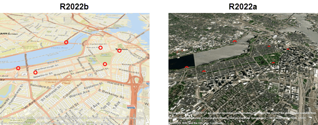
The camera snaps to the plot. In R2023a and earlier releases, the camera flew to the plot. The image on the left shows the camera behavior in R2023a. The image on the right shows the camera behavior in R2023b.


When the data covers a small region, the globe places the camera closer to the plotted data. In R2023a and earlier releases, the globe placed the camera farther away.
When you set the hold state to
"on", then pan or zoom within the globe, and then plot data, the camera does not move. In R2023a and earlier releases, the camera centered on the data. For an example that shows how to preserve the camera view in R2023a and earlier releases, see Preserve Camera View on thecamposreference page.
When you add a plot to a geographic globe by using the geoplot3
function, MATLAB® does not reset the basemap or terrain. In R2022a and earlier releases, the
basemap and terrain reset when you add new plots.
As a result, you can specify the basemap or terrain and then visualize data without
using the hold function. For example, this code creates a globe using
the "streets" basemap and no terrain data. Then, it displays a plot and
adjusts the camera view. In R2022b, the basemap and terrain do not reset. In R2022a and
earlier releases, the basemap reset to the default "satellite" and the
terrain reset to the default "gmted2010".
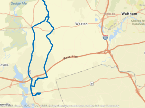
lat = [42.3501 42.3515 42.3598 42.3584 42.3529 42.3626];
lon = [-71.0870 -71.0926 -71.0662 -71.0598 -71.0662 -71.0789];

uif = uifigure;
g = geoglobe(uif,Basemap="streets",Terrain="none");

p = geoplot3(g,lat,lon,0,"ro",LineWidth=3);
campos(g,42.33,-71.0756,2113)
campitch(g,-42.2458)
This change does not affect existing code that sets the hold state to
"on" between commands.
To reset the basemap and terrain, set the Basemap and
Terrain properties to the defaults after you create the plot.
g.Basemap = "satellite";
g.Terrain = "gmted2010";
For more information about changing the basemap and terrain of geographic globes, see Access Basemaps and Terrain for Geographic Globe.
1 Alignment of boundaries and region labels are a presentation of the feature provided by the data vendors and do not imply endorsement by MathWorks®.