Channel Estimation
LTE Toolbox™ uses orthogonal frequency division multiplexing (OFDM) as its digital multicarrier modulation scheme. Channel estimation plays an important part in OFDM systems. It increases the capacity of orthogonal frequency division multiple access (OFDMA) systems by improving the system performance in terms of bit error rate.
To allow estimation of the channel characteristics, LTE uses cell-specific reference signals (pilot symbols) inserted in both time and frequency. These pilot symbols provide an estimate of the channel at given locations within a subframe. Through interpolation, it is possible to estimate the channel across an arbitrary number of subframes.
Channel Estimation Overview
LTE assigns each pilot symbol a position in a subframe depending on the eNodeB cell identification number and which transmit antenna is being used, as shown in this figure.
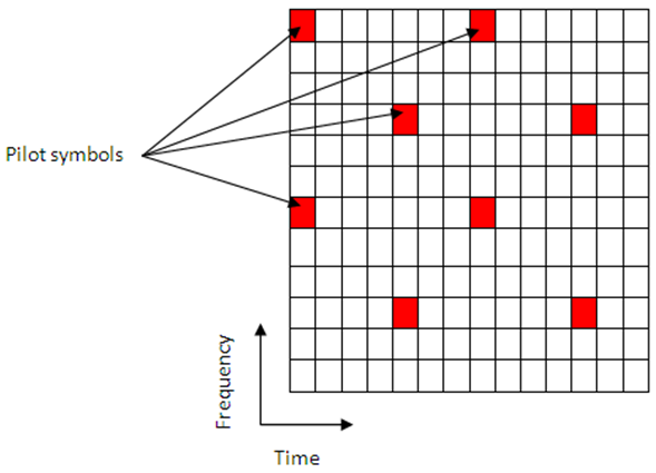
The unique positioning of the pilots ensures that they do not interfere with one another, which enables reliable estimation of the complex gains the propagation channel imparts to the resource elements in the transmitted grid.
This block diagram shows the transmit chain, the propagation channel model, and the receive chain.
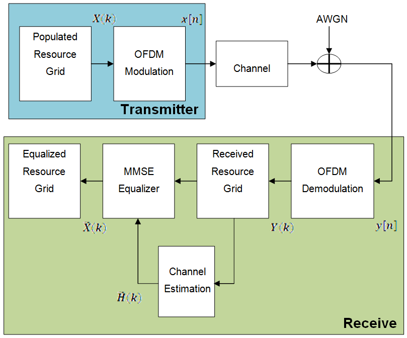
The populated resource grid represents several subframes containing data. The transmitter OFDM-modulates the grid and passes it through the propagation channel model. Channel noise in the form of additive white Gaussian noise (AWGN) is added before the signal enters the receiver. The receiver OFDM-demodulates the signal and constructs a received resource grid. The received resource grid contains the transmitted resource elements which have been affected by the complex channel gains and the channel noise. The receiver can use the known pilot symbols to estimate the channel, then use the channel estimate to equalize the effects of the channel and reduce the noise on the received resource grid.
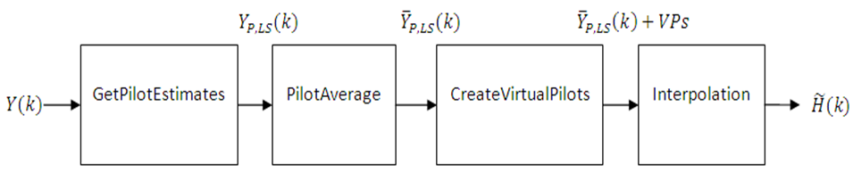
LTE maps reference signals to unique locations within a subframe for each antenna port. Because no other antenna transmits data at these locations in time and frequency, the receiver can perform channel estimation for multi-antenna configurations. The channel estimation algorithm extracts the reference signals for a transmit/receive antenna pair from the received grid. The receiver then calculates the least squares estimates of the channel frequency response at the pilot symbols, as described in On Channel Estimation in OFDM Systems [2]. Then, the receiver averages the least squares estimates to reduce any unwanted noise from the pilot symbols. Because it is possible for no pilots to be located near the subframe edge, virtual pilot symbols are created to aid the interpolation process near the edge of the subframe. Using the averaged pilot symbol estimates and the calculated virtual pilot symbols, the receiver performs interpolation to estimate the entire subframe. The process is shown in this block diagram.
Get Pilot Estimates Subsystem
The first step in determining the least squares estimate is to extract the pilot symbols from their known location within the received subframe. Because the value of these pilot symbols is known, the receiver can determine the channel response at these locations using the least squares estimate. The receiver gets the least squares estimate by dividing the received pilot symbols by their expected value.
Where:
is a received complex symbol value.
is a transmitted complex symbol value.
is a complex channel gain experienced by a symbol.
Known pilot symbols can be sent to estimate the channel for a subset of resource elements (REs) within a subframe. In particular, if pilot symbol is sent in an RE, an instantaneous channel estimate for that RE can be computed using:
Where:
represents the received pilot symbol values.
represents the known transmitted pilot symbol values.
is the true channel response for the RE occupied by the pilot symbol.
Pilot Average Subsystem
To minimize the effects of noise on the channel estimates, the least squares estimates are averaged using an averaging window. This simple method substantially reduces the noise on the pilot REs. You can use the following two pilot symbol averaging methods.
'TestEVM'— follows the method described in TS 36.141 [1], Annex F.3.4.'UserDefined'— allows you to define the window size and direction of averaging used on the pilot symbols plus other settings used for the interpolation.
'TestEVM'
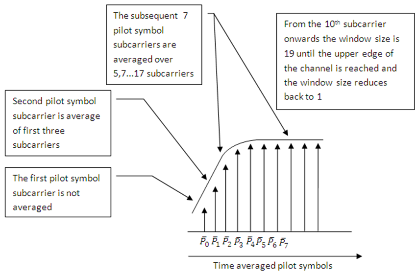
The first method, 'TestEVM', uses the approach described in TS 36.141 [1], Annex F.3.4. The receiver performs time averaging across
each subcarrier that contains a pilot symbol, resulting in a column vector that
contains an average amplitude and phase for each subcarrier that contains a
reference signal.
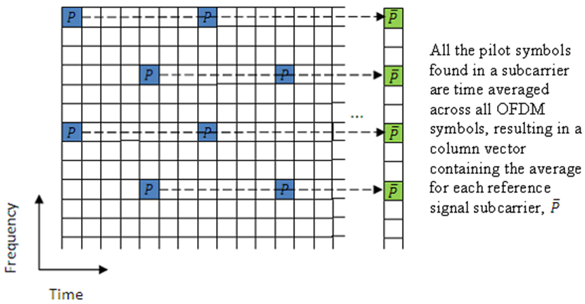
The averages of the pilot symbol subcarriers are then frequency-averaged using a moving window of maximum size 19.
Note
When you use 'TestEVM' pilot symbol averaging there are no
user-defined parameters, so control of channel estimation parameters is not
possible. The estimation is performed using the method described in TS 36.141
[1], except that averaging across 10 subframes is not
strictly required. The lteDLChannelEstimate function
averages across the number of subframes included in the input
rxgrid. The greater the number of subframes in
rxgrid, the more effective the noise averaging in the
time direction.
'UserDefined'
The second pilot symbol averaging method, 'UserDefined', allows you to
define the size of the averaging window, the direction averaging will be done in
(time, frequency or both), and certain aspects of the interpolation that can be
adjusted to suit the available data. For more information, see Interpolation Subsystem.
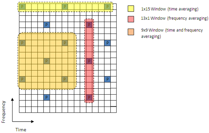
The averaging window size is defined in terms of resource elements. Pilot symbols located within the window are used to average the value of the pilot symbol found at the centre of the window. The window size must be an odd number: this ensures that there is a pilot at the center.
Note
Averaging the channel estimates at pilot symbol locations is a simple, powerful tool, but you must choose the window size carefully. Using a large window size on a fast fading channel could result in averaging out not only noise, but also channel characteristics. Performing too much averaging on a system with a small amount of noise can have an adverse effect on the quality of the channel estimates. Therefore, using a large averaging window for a fast changing channel could cause the estimate of the channel to appear flat, resulting in a poor estimate of the channel and affecting the quality of the equalization.
Create Virtual Pilots Subsystem
In many cases, the edges of the resource grid do not contain any pilot symbols. This is shown in this figure.
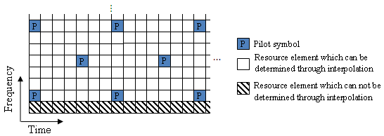
In this case, channel estimates at the edges cannot be interpolated from the pilot symbols. To
overcome this problem, virtual pilot symbols are created. The lteDLChannelEstimate function creates virtual pilot symbols on all the
edges of the received grid to allow cubic interpolation.
Virtual Pilot Placement
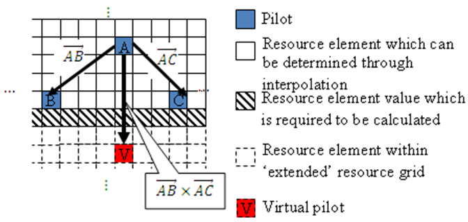
Virtual pilot symbols are created, as shown in this figure.
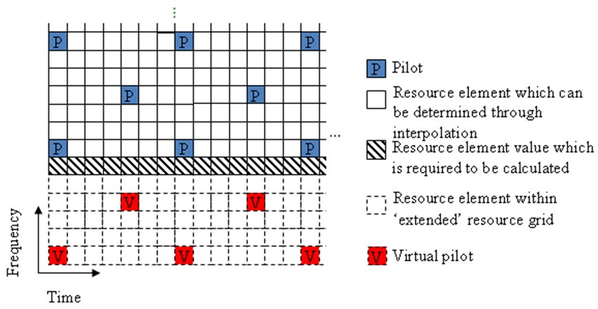
In this system, the resource grid is extended, with virtual pilot symbols created in locations that follow the original reference signal pattern. The virtual pilot symbols allow the channel estimate to be calculated by interpolation.
Calculating Virtual Pilot Symbol Values
The virtual pilot symbols are calculated using the original pilot symbols. The receiver calculates the value of the virtual pilot symbols by following these steps:
Choose the 10 closest original pilots in Euclidean distance in time and frequency. The search is optimized to consider these 10 pilots, rather than checking all possible pilots. Based on the possible configurations of the cell reference signal, using 10 pilots provides sufficient time and frequency diversity for the virtual pilot calculation.
From the 10 pilots, choose the three closest pilot symbols. These three symbols must occupy at least two unique subcarriers and two unique OFDM symbols.
Using this set of three pilots, create two vectors: one between the closest and furthest pilot symbols, and one between the second-closest and furthest pilot symbols.
Calculate the cross product of the two vectors to create a plane on which the three points reside.
Extend the plane to the position of the virtual pilot to calculate the value based on one of the actual pilot values.
This diagram shows the virtual pilot calculation.
Note
Virtual pilots are only created for the MATLAB® 'linear' and 'cubic' interpolation
methods.
Interpolation Subsystem
Once the receiver has removed or reduced the noise from the least squares pilot symbol
averages and sufficient virtual pilots have been determined, you can use interpolation
to estimate the missing values from the channel estimation grid. The lteDLChannelEstimate function has two pilot symbol averaging methods,
'TestEVM' and 'UserDefined'. The pilot symbol
averaging methods also define the interpolation method the function uses to obtain the
channel estimate.
The 'TestEVM' pilot averaging method described in TS 36.141 [1], Annex F.3.4, requires the use of simple linear interpolation on
the time-averaged and frequency-averaged column vector. The interpolation is
one-dimensional, since it only estimates the values between the averaged pilot symbol
subcarriers in the column vector. The function replicates the resulting vector and uses
it as the channel estimate for the entire resource grid.
The 'UserDefined' pilot averaging method performs two-dimensional
interpolation to estimate the channel response between the available pilot symbols. The
function uses an interpolation window to specify which data is used to perform the
interpolation. The InterpWindow field defines the causal nature of
the available data. The valid settings for
cec.InterpWindow are
'Causal', 'Non-causal', and
'Centered'.
Use the InterpWindow setting:
'Causal'when using past data.'Non-causal'when using future data. Relying only on future data is commonly referred to as an anti-causal method of interpolation.'Centered'or'Centred'when using a combination of past, present, and future data.
The size of the interpolation window can also be adjusted to suit the available data. To
specify the window size, set the InterpWinSize field.
Noise Estimation
The performance of some receivers can be improved using knowledge of the noise power of the
received signal. The lteDLChannelEstimate function provides an
estimate of the noise power spectral density (PSD) using the estimated channel response
at known reference signal locations. The noise power can be determined by analyzing the
noisy least squares estimates and the noise-averaged estimates.
The noisy least squares estimates from the Get Pilot Estimates Subsystem and the noise-averaged pilot symbol estimates from the Pilot Average Subsystem provide an indication of the channel noise. The least squares estimates and the averaged estimates contain the same data, except for additive noise. Taking the difference of the two estimates results in a noise level value for the least squares channel estimates at pilot symbol locations. Considering again,
Averaging the instantaneous channel estimates over the smoothing window gives
where S is the set of pilots in the smoothing window and |S| is the number of pilots in S. Therefore, an estimate of the noise at a particular pilot RE is given by:
In practice, it is not possible to remove all the noise using averaging. Because it is only possible to reduce the noise, only an estimate of the noise power can be made.
Note
In the case of a noiseless system or a system with a high SNR, averaging could worsen the least squares estimates.
Using the value of the noise power found in the channel response at pilot symbol locations, the noise power per resource element (RE) can be calculated by taking the variance of the resulting noise vector. The noise power per RE for each transmit and receive antenna pair is calculated and stored. The mean of this matrix is returned as the estimate of the noise power per RE.
For a demonstration on how to set up a full transmit and receive chain for channel estimation, see PDSCH Transmit Diversity Throughput Simulation. In this example, multiple antennas are used and transmission is simulated through a propagation channel model.
References
[1] 3GPP TS 36.141. “Evolved Universal Terrestrial Radio Access (E-UTRA); Base Station (BS) Conformance Testing.” 3rd Generation Partnership Project; Technical Specification Group Radio Access Network. URL: https://www.3gpp.org.
[2] Van de Beek, J.-J., O. Edfors, M. Sandell, S. K. Wilson, and P. O. Borjesson. “On Channel Estimation in OFDM Systems." Vehicular Technology Conference, IEEE 45th, Volume 2, IEEE, 1995.
See Also
lteDLChannelEstimate | lteEqualizeMMSE | lteEqualizeZF | lteOFDMDemodulate