복소수 데이터를 사용한 스펙트럼 추정 - Marple의 테스트 케이스

라이브 스크립트 열기

이 예제에서는 시계열 데이터에서 스펙트럼 추정을 수행하는 방법을 보여줍니다. Marple의 테스트 케이스(The complex data in L. Marple: S.L. Marple, Jr, Digital Spectral Analysis with Applications, Prentice-Hall, Englewood Cliffs, NJ 1987.)를 사용합니다.

테스트 데이터

테스트 데이터를 불러와 시작합니다.

load marple

System Identification Toolbox™의 루틴은 대부분 복소수 데이터를 지원합니다. 하지만 플로팅을 위해 데이터의 실수부와 허수부를 따로 검사하겠습니다.

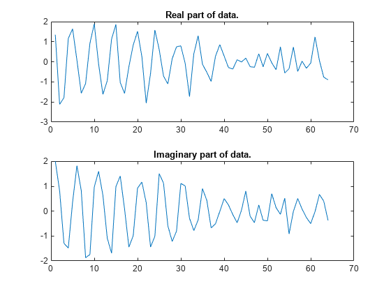
먼저 데이터를 살펴봅니다.

subplot(211),plot(real(marple)),title('Real part of data.')
subplot(212),plot(imag(marple)),title('Imaginary part of data.')

Figure contains 2 axes objects. Axes object 1 with title Real part of data. contains an object of type line. Axes object 2 with title Imaginary part of data. contains an object of type line.

예비 분석 단계로, 데이터 주기도를 검사해 보겠습니다.

per = etfe(marple);
w = per.Frequency;
clf
h = spectrumplot(per,w);
opt = getoptions(h);
opt.FreqScale = 'linear';
opt.FreqUnits = 'Hz';
setoptions(h,opt)

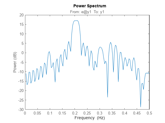
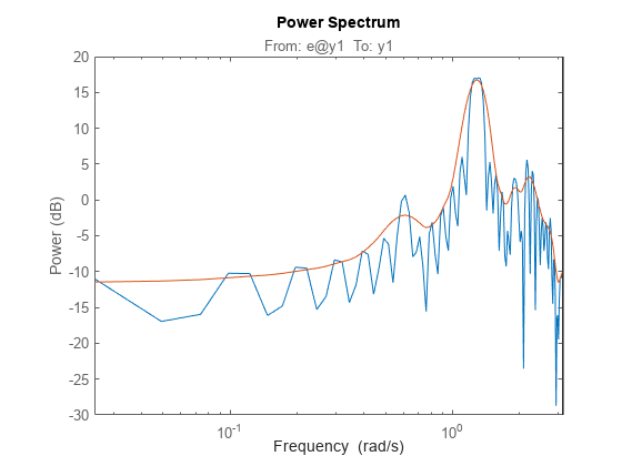
Figure contains an axes object. The axes object with title From: e@y1 To: y1, ylabel Power (dB) contains an object of type line. This object represents per.

데이터 레코드는 64개 샘플뿐이고 주기도는 128개 주파수에 대해 계산되었기 때문에 좁은 주파수 윈도우에서 진동을 명확하게 확인할 수 있습니다. 따라서 주기도에 평활화를 적용합니다(1/32Hz의 주파수 분해능에 해당).

sp = etfe(marple,32);
spectrumplot(per,sp,w);

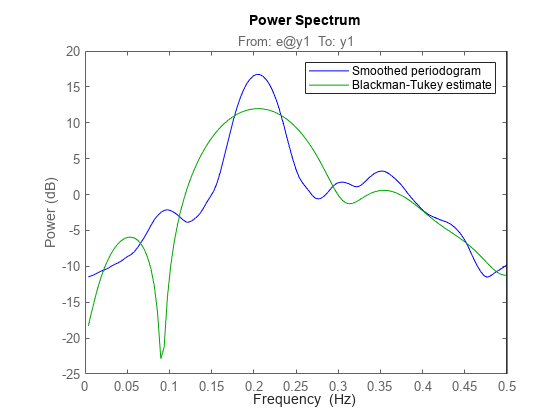
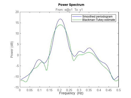
Figure contains an axes object. The axes object with title From: e@y1 To: y1, ylabel Power (dB) contains 2 objects of type line. These objects represent per, sp.

이제 블랙맨-튜키(Blackman-Tukey) 방법을 스펙트럼 추정에 사용해 보겠습니다.

ssm = spa(marple); % Function spa performs spectral estimation
spectrumplot(sp,'b',ssm,'g',w,opt);    
legend({'Smoothed periodogram','Blackman-Tukey estimate'});

Figure contains an axes object. The axes object with title From: e@y1 To: y1, ylabel Power (dB) contains 2 objects of type line. These objects represent Smoothed periodogram, Blackman-Tukey estimate.

디폴트 윈도우 길이는 이 소량의 데이터에 대해 매우 좁은 지연 윈도우를 제공합니다. 다음 방법으로 더 큰 지연 윈도우를 선택할 수 있습니다.

ss20 = spa(marple,20);
spectrumplot(sp,'b',ss20,'g',w,opt);
legend({'Smoothed periodogram','Blackman-Tukey estimate'});

Figure contains an axes object. The axes object with title From: e@y1 To: y1, ylabel Power (dB) contains 2 objects of type line. These objects represent Smoothed periodogram, Blackman-Tukey estimate.

자기회귀(AR) 모델 추정하기

모수적 5차 AR 모델은 다음과 같이 계산됩니다.

t5 = ar(marple,5);

주기도 추정값과 비교합니다.

spectrumplot(sp,'b',t5,'g',w,opt); 
legend({'Smoothed periodogram','5th order AR estimate'});

Figure contains an axes object. The axes object with title From: e@y1 To: y1, ylabel Power (dB) contains 2 objects of type line. These objects represent Smoothed periodogram, 5th order AR estimate.

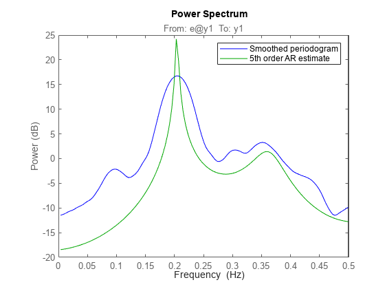
사실상 AR 명령은 스펙트럼 추정을 위한 20개의 서로 다른 방법을 포함합니다. 위에 나온 방법은 Marple 교재에서 '수정된 공분산 추정값(the modified covariance estimate)'으로 알려져 있습니다.

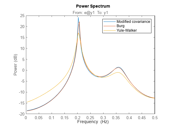
잘 알려진 몇 가지 다른 방법의 결과는 다음과 같이 얻습니다.

tb5 = ar(marple,5,'burg');      % Burg's method
ty5 = ar(marple,5,'yw');        % The Yule-Walker method
spectrumplot(t5,tb5,ty5,w,opt);
legend({'Modified covariance','Burg','Yule-Walker'})

Figure contains an axes object. The axes object with title From: e@y1 To: y1, ylabel Power (dB) contains 3 objects of type line. These objects represent Modified covariance, Burg, Yule-Walker.

도구 변수 방법을 사용하여 AR 모델 추정하기

AR 모델링은 도구 변수 방법을 사용하여 수행할 수도 있습니다. 이를 위해 여기서는 ivar 함수를 사용합니다.

ti = ivar(marple,4); 
spectrumplot(t5,ti,w,opt);
legend({'Modified covariance','Instrumental Variable'})

Figure contains an axes object. The axes object with title From: e@y1 To: y1, ylabel Power (dB) contains 2 objects of type line. These objects represent Modified covariance, Instrumental Variable.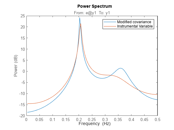

스펙트럼의 자기회귀 이동평균(ARMA) 모델

아울러 System Identification Toolbox에는 스펙트럼의 ARMA 모델링도 포함됩니다.

ta44 = armax(marple,[4 4]); % 4 AR-parameters and 4 MA-parameters
spectrumplot(t5,ta44,w,opt);
legend({'Modified covariance','ARMA'})

Figure contains an axes object. The axes object with title From: e@y1 To: y1, ylabel Power (dB) contains 2 objects of type line. These objects represent Modified covariance, ARMA.