Examine Model Residuals
This example shows how you can use residual analysis to evaluate model quality.
Creating Residual Plots
To load the sample System Identification app session that contains estimated models, type the following command in the MATLAB® Command Window:
systemIdentification('dryer2_linear_models')To generate a residual analysis plot, select the Model resids check box in the System Identification app.
This opens an empty plot.
In the System Identification app window, click each parametric model icon to display it on the Residual Analysis plot. Do not click the nonparametric model
spad, as residual analysis plots are not available for this model.
Description of the Residual Plot Axes
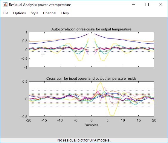
The top axes show the autocorrelation of residuals for the output (whiteness test). The
horizontal scale is the number of lags, which is the time difference (in samples) between the
signals at which the correlation is estimated. The horizontal dashed lines on the plot represent
the confidence interval of the corresponding estimates. Any fluctuations within the confidence
interval are considered to be insignificant. Six of the models —arxqs,
n4s3, arx223,
tf1,ss1, and amx2222 — produce
residuals that enter outside the confidence interval. A good model should have a residual
autocorrelation function within the confidence interval, indicating that the residuals are
uncorrelated.
The bottom axes show the cross-correlation of the residuals
with the input. A good model should have residuals uncorrelated with
past inputs (independence test). Evidence of correlation indicates
that the model does not describe how the output is formed from the
corresponding input. For example, when there is a peak outside the
confidence interval for lag k, this means that
the contribution to the output y(t) that originates
from the input u(t-k) is not properly described
by the model. The models arxqs and amx2222 extend
beyond the confidence interval and do not perform as well as the other
models.
Validating Models Using Analyzing Residuals
To remove models with poor performance from the Residual Analysis plot, click the model icons
arxqs, n4s3, arx223,
tf1, ss1, and amx2222 in the System
Identification app.
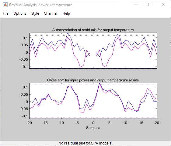
The Residual Analysis plot now includes only the two models that pass the residual tests:
arx692 and amx3322.

The plots for these models fall primarily within the confidence intervals, although the
amx3322 plot shows some excursions slightly outside of the boundaries. If
these excursions are acceptable, it is reasonable to pick the amx3322 model
because it is a simpler low-order model. If the excursions are not acceptable, you can use the
arx392 model instead.