Estimating Simple Models from Real Laboratory Process Data
This example shows how to develop and analyze simple models from a real laboratory process data. We start with a small description of the process, learn how to import the data to the toolbox and preprocess/condition it and then proceed systematically to estimate parametric and nonparametric models. Once the models have been identified we compare the estimated models and also validate the model to the actual output data from the experiment.
System Description
This case study concerns data collected from a laboratory scale "hairdryer". (Feedback's Process Trainer PT326; See also page 525 in Ljung, 1999). The process works as follows: Air is fanned through a tube and heated at the inlet. The air temperature is measured by a thermocouple at the outlet. The input is the voltage over the heating device, which is just a mesh of resistor wires. The output is the outlet air temperature represented by the measured thermocouple voltage.
Setting Up Data for Analysis
First we load the input-output data to the MATLAB® Workspace.
load dryer2;
Vector y2, the output, contains 1000 measurements of the thermocouple voltage which is proportional to the temperature in the outlet airstream. Vector u2 contains 1000 input data points consisting of the voltage applied to the heater. The input was generated as a binary random sequence that switches from one level to the other with probability 0.2. The sample time is 0.08 seconds.
The next step is to set up the data as an iddata object.
dry = iddata(y2,u2,0.08);
To get information about the data, just type the name of the iddata object at the MATLAB command window:
dry
dry =

Time domain data set with 1000 samples.
Sample time: 0.08 seconds

Outputs      Unit (if specified)
   y1

Inputs       Unit (if specified)
   u1
To inspect the properties of the above iddata object, use the get command:
get(dry)
ans =

  struct with fields:

              Domain: 'Time'
                Name: ''
          OutputData: [1000×1 double]
          OutputName: {'y1'}
          OutputUnit: {''}
           InputData: [1000×1 double]
           InputName: {'u1'}
           InputUnit: {''}
              Period: Inf
         InterSample: 'zoh'
                  Ts: 0.0800
              Tstart: 0.0800
    SamplingInstants: [1000×1 double]
            TimeUnit: 'seconds'
      ExperimentName: 'Exp1'
               Notes: [0×1 string]
            UserData: []
For better book-keeping, it is good practice to give names to the input and output channels and Time units. These names would be propagated throughout the analysis of this iddata object:
dry.InputName = 'Heater Voltage';
dry.OutputName = 'Thermocouple Voltage';
dry.TimeUnit = 'seconds';
dry.InputUnit = 'V';
dry.OutputUnit = 'V';
Now that we have the data set ready, we choose the first 300 data points for model estimation.
ze = dry(1:300)
ze =

Time domain data set with 300 samples.
Sample time: 0.08 seconds

Outputs                    Unit (if specified)
   Thermocouple Voltage       V

Inputs                     Unit (if specified)
   Heater Voltage             V
Preprocessing the Data
Plot the interval from sample 200 to 300:
plot(ze(200:300));
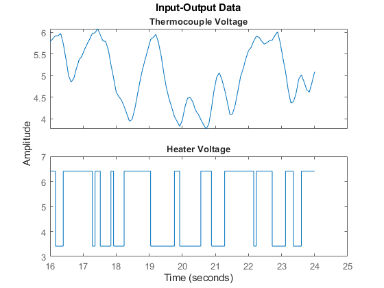
Figure 1: A snapshot of the measured hair-dryer data.
From the above plot, it can be observed that the data is not zero mean. So let us remove the constant levels and make the data zero mean.
ze = detrend(ze);
The same data set after it has been detrended:
plot(ze(200:300)) %show samples from 200 to 300 of detrended data
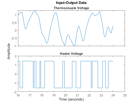
Figure 2: Detrended estimation data.
Estimating Nonparametric and Parametric Models
Now that the dataset has been detrended and there are no obvious outliers, let us first estimate the impulse response of the system by correlation analysis to get some idea of time constants and the like:
clf
mi = impulseest(ze); % non-parametric (FIR) model
showConfidence(impulseplot(mi),3); %impulse response with 3 standard
                                   %deviations confidence region
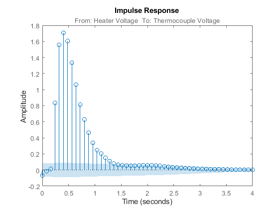
Figure 3: Impulse response of the FIR model estimated using ze.
The shaded region marks a 99.7% confidence interval. There is a time delay (dead-time) of 3 samples before the output responds to the input (significant output outside the confidence interval).
The simplest way to get started on a parametric estimation routine is to build a state-space model where the model-order is automatically determined, using a prediction error method. Let us estimate a model using the ssest estimation technique:
m1 = ssest(ze);
m1 is a continuous-time identified state-space model, represented by an idss object. The estimation algorithm chooses 3 as the optimal order of the model. To inspect the properties of the estimated model, just enter the model name at the command window:
m1
m1 =
  Continuous-time identified state-space model:
      dx/dt = A x(t) + B u(t) + K e(t)
       y(t) = C x(t) + D u(t) + e(t)

  A =
            x1       x2       x3
   x1  -0.4839   -2.011   -2.092
   x2    3.321   -1.913   -5.998
   x3   -1.623    17.01   -15.61

  B =
       Heater Volta
   x1      -0.05753
   x2       0.02004
   x3        -1.377

  C =
                       x1        x2        x3
   Thermocouple    -14.07   0.07729  -0.04252

  D =
                 Heater Volta
   Thermocouple             0

  K =
       Thermocouple
   x1       -0.9457
   x2      -0.02097
   x3        -2.102

Parameterization:
   FREE form (all coefficients in A, B, C free).
   Feedthrough: none
   Disturbance component: estimate
   Number of free coefficients: 18
   Use "idssdata", "getpvec", "getcov" for parameters and their uncertainties.

Status:
Estimated using SSEST on time domain data "ze".
Fit to estimation data: 95.32% (prediction focus)
FPE: 0.001621, MSE: 0.001526
The display suggests that the model is free-form (all entries of A, B and C matrices were treated as free parameters) and that the estimated model fits the data pretty well (over 90% fit). To retrieve the properties of this model, for example to obtain the A matrix of the discrete state-space object generated above, we can use the dot operator:
A = m1.a;
See the "Data and Model Objects in System Identification Toolbox" example for more information regarding model objects. To find out which properties of the model object can be retrieved, use get command:
get(m1)
                A: [3×3 double]
                B: [3×1 double]
                C: [-14.0706 0.0773 -0.0425]
                D: 0
                K: [3×1 double]
        StateName: {3×1 cell}
        StateUnit: {3×1 cell}
        Structure: [1×1 pmodel.ss]
    NoiseVariance: 1.2587e-04
       InputDelay: 0
      OutputDelay: 0
        InputName: {'Heater Voltage'}
        InputUnit: {'V'}
       InputGroup: [1×1 struct]
       OutputName: {'Thermocouple Voltage'}
       OutputUnit: {'V'}
      OutputGroup: [1×1 struct]
            Notes: [0×1 string]
         UserData: []
             Name: ''
               Ts: 0
         TimeUnit: 'seconds'
     SamplingGrid: [1×1 struct]
           Report: [1×1 idresults.ssest]
To fetch the values of the state-space matrices and their 1 standard deviation uncertainties, use the idssdata command:
[A,B,C,D,K,~,dA,dB,dC,dD,dK] = idssdata(m1)
A =

   -0.4839   -2.0112   -2.0917
    3.3205   -1.9135   -5.9981
   -1.6235   17.0096  -15.6070


B =

   -0.0575
    0.0200
   -1.3770


C =

  -14.0706    0.0773   -0.0425


D =

     0


K =

   -0.9457
   -0.0210
   -2.1019


dA =

   1.0e+15 *

    0.1488    0.1279    0.1186
    0.2932    0.2775    0.2394
    1.2099    0.8557    0.3205


dB =

   1.0e+13 *

    0.5677
    1.9832
    5.8673


dC =

   1.0e+14 *

    2.8857    1.9809    0.6024


dD =

     0


dK =

   1.0e+13 *

    1.8409
    4.9993
    9.9641
The uncertainties are quite large even though the model fit the estimation data well. This is because the model is over-parameterized, that is, it has more free parameters than what could be uniquely identified. The variance of parameters in such cases is not well defined. However this does not imply that the model is unreliable. We can plot the time- and frequency-response of this plot and view the variance as confidence regions as discussed next.
Analyzing the Estimated Model
The Bode plot of the generated model can be obtained using the bode function as shown below:
h = bodeplot(m1);

Figure 4: Bode plot of estimated model.
Right-click on the plot and pick Characteristics->Confidence Region. Or, use the showConfidence command to view the variance of the response.
showConfidence(h,3) % 3 standard deviation (99.7%) confidence region
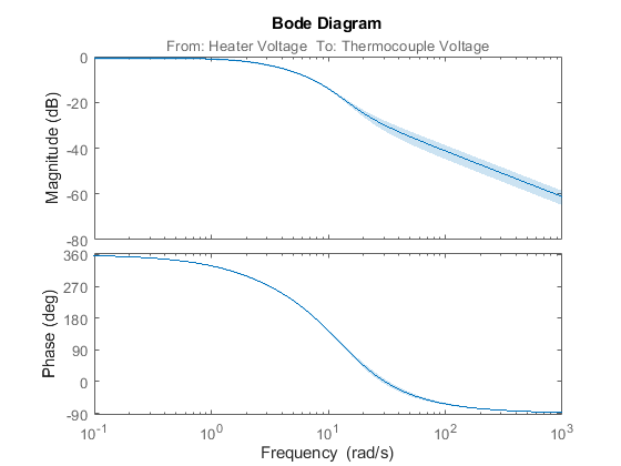
Figure 5: Bode plot with 3 standard deviation confidence region.
Similarly, we can generate the step plot and its associated 3 standard deviation confidence region. We can compare the responses and associated variances of the parametric model m1 with that of the nonparametric model mi:
showConfidence(stepplot(m1,'b',mi,'r',3),3)

Figure 6: Step plot of models m1 and mi with confidence regions.
We can also consider the Nyquist plot, and mark uncertainty regions at certain frequencies with ellipses, corresponding to 3 standard deviations:
Opt = nyquistoptions;
Opt.ShowFullContour = 'off';
showConfidence(nyquistplot(m1,Opt),3)

Figure 7: Nyquist plot of estimated model showing the uncertainty regions at certain frequencies.
The response plots show that the estimated model m1 is quite reliable.
Estimating Models with a Prescribed Structure
System Identification Toolbox™ can also be used to obtain a model with a prescribed structure. For example, a difference equation model with 2 poles, 1 zero and 3 sample delays can be obtained using the arx function as shown below:
m2 = arx(ze,[2 2 3]);
To look at the model, enter the model name at the command window.
m2
m2 =
Discrete-time ARX model: A(z)y(t) = B(z)u(t) + e(t)
  A(z) = 1 - 1.274 z^-1 + 0.3942 z^-2

  B(z) = 0.06679 z^-3 + 0.04429 z^-4

Sample time: 0.08 seconds

Parameterization:
   Polynomial orders:   na=2   nb=2   nk=3
   Number of free coefficients: 4
   Use "polydata", "getpvec", "getcov" for parameters and their uncertainties.

Status:
Estimated using ARX on time domain data "ze".
Fit to estimation data: 95.08% (prediction focus)
FPE: 0.001756, MSE: 0.001687
A continuous time transfer function with 2 poles, one zero and 0.2 second transport delay can be estimated using the tfest command:
m3 = tfest(ze, 2, 1, 0.2)
m3 =

  From input "Heater Voltage" to output "Thermocouple Voltage":
                   1.183 s + 26.55
  exp(-0.2*s) * ---------------------
                s^2 + 11.61 s + 28.63

Continuous-time identified transfer function.

Parameterization:
   Number of poles: 2   Number of zeros: 1
   Number of free coefficients: 4
   Use "tfdata", "getpvec", "getcov" for parameters and their uncertainties.

Status:
Estimated using TFEST on time domain data "ze".
Fit to estimation data: 88.79%
FPE: 0.009126, MSE: 0.008768
Validating the Estimated Model to Experimental Output
How good is an estimated model? One way to find out is to simulate it and compare the model output with measured output. Select a portion of the original data that was not used in building the model, say from samples 800 to 900. Once the validation data has been preprocessed, we use the compare function as shown below to view the quality of prediction:
zv = dry(800:900);   % select an independent data set for validation
zv = detrend(zv);    % preprocess the validation data
set(gcf,'DefaultLegendLocation','best')
compare(zv,m1);      % perform comparison of simulated output
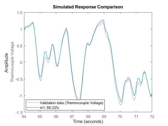
Figure 8: Model's simulated response vs. validation data output.
It can be observed here that the agreement is very good. The "Fit" value shown is calculated as:
Fit = 100*(1 - norm(yh - y)/norm(y-mean(y)))
where y is the measured output (=|zv.y|), and yh is the output of the model m1.
Comparing Estimated Models
To compare the performance of the models that we have estimated, for example m1, m2 and m3 with the validation data zv, we can again use the compare command:
compare(zv,m1,'b',m2,'r',m3,'c');
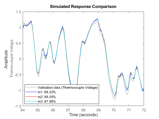
Figure 9: Comparing the responses of models m1, m2, m3 on validation data set ze.
As m3 is a continuous-time system, use pade function to approximate the transport delay. You can then obtain the pole-zero plots for the models using iopzplot:
m3x = pade(m3,2);
h = iopzplot(m1,'b',m2,'r',m3x,'c');
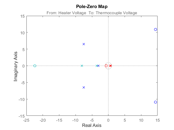
Figure 10: Poles and zeros of the models m1, m2 and m3.
The uncertainties in the poles and zeros can also be obtained. In the following statement, '3' refers to the number of standard deviations.
showConfidence(h,3);
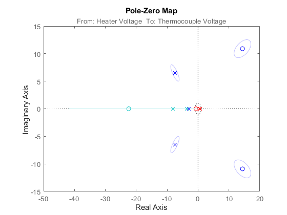
Figure 11: Pole-zero map with uncertainty regions.
The frequency functions above that are obtained from the models can be compared with one that is obtained using a non-parametric spectral analysis method (spa):
gs = spa(ze);
The spa command produces an IDFRD model. The bode function can again be used for a comparison with the transfer functions of the models obtained.
w = linspace(0.4,pi/m2.Ts,200);
opt = bodeoptions; opt.PhaseMatching = 'on';
bodeplot(m1,'b',m2,'r',m3,'c',gs,'g',w,opt);
legend('m1','m2','m3','gs')
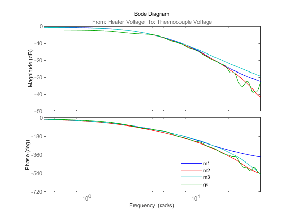
Figure 12: Bode responses of m1, m2 and m3 compared against the non-parametric spectral estimation model gs.
The frequency responses from the three models/methods are very close. This indicates that this response is reliable.
Also, a Nyquist plot can be analyzed with the uncertainty regions marked at certain frequencies:
showConfidence(nyquistplot(m1,'b',m2,'r',m3,'c',gs,'g'),3)
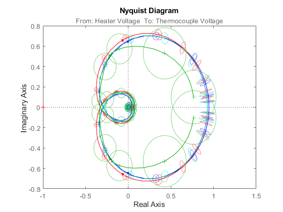
Figure 13: Nyquist plots of models m1, m2, m3 and gs.
The non-parametric model gs exhibits the most uncertainty in response.