Model a Refrigeration Cycle

R2026b

This example explains how to model a closed-loop refrigeration cycle. Simulating a refrigeration cycle requires you to properly tune the component parameters. Imbalances in the net energy transfer can cause runaway system pressure and temperature. Because the refrigerant undergoes energy transfer that causes substantial and rapid density changes, you start by modeling and verifying the response of the individual components. You integrate the components into an open-loop system, and then close the loop.

This example develops the model from the Refrigeration Cycle (Air Conditioning) example. In this example, you:

1. Use a P-H Diagram (2P) block to define the operating region of your refrigeration system.

2. Build a test harness for the evaporator using the System-Level Condenser Evaporator (2P-MA) block with an ideal flow source and reservoir blocks for boundary conditions.

3. Substitute a Thermostatic Expansion Valve (2P) block into the evaporator test harness.

4. Build a test harness for the condenser using the System-Level Condenser Evaporator (2P-MA) block with a Positive-Displacement Compressor (2P) block, and use two-phase and moist air reservoir blocks for the boundary conditions.

5. Use a Receiver Accumulator (2P) block to connect the harness from step 3 to the harness from step 4.

6. Remove two-phase reservoir blocks and connect the systems before verifying your results.

After each step, test the components at the desired steady-state nominal conditions to make sure the components are stable and the results are what you expect.

After you assemble a stable refrigeration cycle model, you can simulate conditions beyond nominal values by adjusting the reservoir blocks that represent the environment. Keep the nominal parameters in the model component the same, as they represent the nominal sizing of the component.

Step 1: Determine the Pressure-Enthalpy Diagram

You must define parameters for the evaporator, condenser, thermostatic expansion valve, and receiver-accumulator. Before you can define these parameters, you must create a pressure-enthalpy diagram for the refrigeration cycle.

1. Determine the nominal operating conditions for the system based on your design requirements. This example uses these requirements:

Condition	Setting
Ambient temperature	30 °C
Desired indoor temperature	22 °C
Area of the house	200 m$${}^2$$
Cooling capacity	16 kW or 4.5 tons of refrigeration

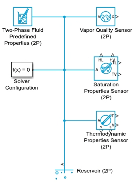
2. In the model, connect a Solver Configuration block and a Reservoir (2P) block to a Two-Phase Fluid Predefined Properties (2P) block.

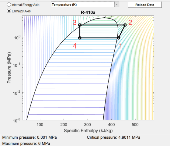
3. Choose the appropriate refrigerant for your design requirements. The example model uses R-410a. Then, generate a P-h diagram for that refrigerant and select the four points of the refrigeration cycle. To plot fluid property contours on a pressure-enthalpy diagram, open the Two-Phase Fluid Predefined Properties (2P) or Two-Phase Fluid Properties (2P) block dialog box. Click the Plot button next to Two-phase fluid properties (contours). Then, select Enthalpy x-axis. Mouse over the data points in the diagram to see information about the pressure, specific enthalpy, and temperature contour values.

4. To enable heat transfer from the refrigerant to the outdoor environment, set the condensing temperature, or the saturation temperature in the condenser, to be higher than the outdoor temperature. The example model uses a 45 °C refrigerant temperature to provide a 15 °C temperature difference with ambient.

5. To enable heat transfer from the indoor air to the refrigerant, set the evaporating temperature, or the saturation temperature in the evaporator, to be lower than the desired indoor temperature. The example model uses a 5 °C evaporator refrigerant inlet temperature to remove heat from the 22 °C house.

6. To estimate the end points of the specific enthalpy for the high- and low-pressure lines in the cycle, set the amount of subcooling at the condenser outlet.

7. Compile the information to find estimates for the four points of the P-h diagram. The example model uses these values:

Location	Point Number	Pressure (p)	Specific Enthalpy (h)	Notes
Evaporator outlet	1	0.934 MPa	430 kJ/kg	Corresponds to a superheat of 5 °C
Condenser inlet	2	2.734 MPa	457 kJ/kg	Corresponds to an estimated temperature of 65 °C
Condenser outlet	3	2.734 MPa	267 kJ/kg	Corresponds to a subcooling of 5 °C
Evaporator inlet	4	0.934 MPa	267 kJ/kg	Corresponds to a vapor quality of 0.27

As you develop and refine your model, you can modify these values to be more accurate or precise.

8. Draw the four points onto the refrigerant P-h plot. In MATLAB, enter:

hold on

plot([430 457 267 267 430], [0.934 2.734 2.734 0.934 0.934], 'k-o', LineWidth = 2)

You can also use a simple model with reservoirs and the desired sensor blocks to determine the P-h diagram.

• There is no flow to or from the reservoir, so sensor blocks measure fluid property values in the reservoir.

• Adjust the conditions as needed to get fluid property values at different conditions from the sensors.

To view the example model created in this step, enter:

ModelARefrigerationCycleStep1

For more information on building a P-h diagram from your operating points, see Identify Refrigeration Cycle Operating Points.

Step 2: Set Up the Evaporator Test Harness

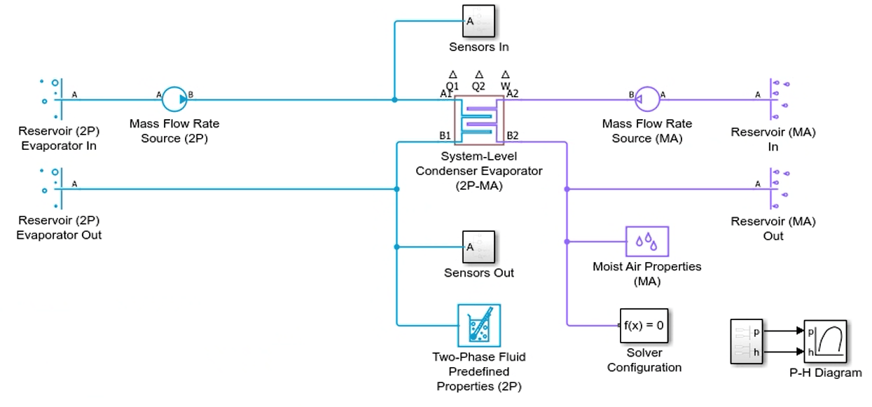
Next, represent the evaporator interaction between the refrigerant and the volume of air in the house. Build the test harness around a System-Level Condenser Evaporator (2P-MA) block. Represent the boundary conditions with the Reservoir (2P) and Reservoir (MA) blocks. Parameterize these blocks using the values you chose in step 1.

1. To model the refrigerant mass flow rate, add a Flow Rate Source (2P) block. To model the air mass flow rate, add a Flow Rate Source (MA) block. Set the Source type parameter to Constant for both blocks. Because both blocks represent boundary conditions that do no work on the flow, set the Power added parameter to None.

2. To approximate mass flow rate values for step 2, use the information from step 1. To approximate the mass flow rate value for the:

• Refrigerant — Use the equation $$Q=\underset{}{\overset{\dot{}}{m}}\Delta h$$ to solve for the mass flow rate. Divide the cooling capacity by the difference between the evaporator outlet specific enthalpy and the evaporator inlet specific enthalpy. For this example, the mass flow rate is 16 kW / (430 kJ/kg - 267 kJ/kg) = 0.1 kg/s.

• Air — Use the equation $$Q=\underset{}{\overset{\dot{}}{m}}{C}_p\Delta T$$ to solve for the mass flow rate. Divide the cooling capacity by the pressure coefficient of air, and divide that result by the desired temperature drop across the evaporator. For this example, the temperature drop is 10 °C, which is equivalent to a temperature drop of 10 K. Consequently, 16 kW / 1 kg/kJ/K / 10 K = 1.6 kg/s. To calculate the volumetric flow rate, divide the mass flow rate of the air by the density of air. For this example, the value is 1.6 kg/s / 1.2 kg/m = 1.33 m$${}^3$$/s.

3. Run the simulation and check your results by using Simscape Results Explorer. The simulation should be close to steady-state. Check that the simulation outputs match your conditions from step 1.

4. If the simulation outputs do not match the P-h diagram conditions, adjust the mass flow rate for both the Flow Rate Source (2P) block and the System-Level Condenser Evaporator (2P-MA) blocks. You can use a Condenser Evaporator (2P-MA) block to obtain a higher fidelity model, but you should first validate your model with the System-Level Condenser Evaporator (2P-MA) block.

5. Adjust the mass flow rate for the Flow Rate Source (MA) and System-Level Condenser Evaporator (2P-MA) blocks until your model meets the P-h diagram conditions. The example model uses a volumetric flow rate of 1.33 m$${}^3$$/s. This flow rate corresponds to a temperature drop of about 9 °C across the evaporator, where the return air is 24 °C and the supply air is about 15 °C. The air does not achieve the full 10 °C temperature drop calculated with the simplified $$Q=\underset{}{\overset{\dot{}}{m}}{C}_p\Delta T$$ equation because of a small amount of water condensation inside the heat exchanger.

6. Choose an appropriate refrigerant tube size based on the refrigerant mass flow rate.

7. Choose an appropriate air duct size based on the air flow rate.

To view the example model created in this step, enter:

ModelARefrigerationCycleStep2

Step 3: Set Up the Thermostatic Expansion Valve Test Harness

Next, model a thermostatic expansion valve that controls the performance of the evaporator. A thermostatic expansion valve modulates the flow into the evaporator based on the measured superheat.

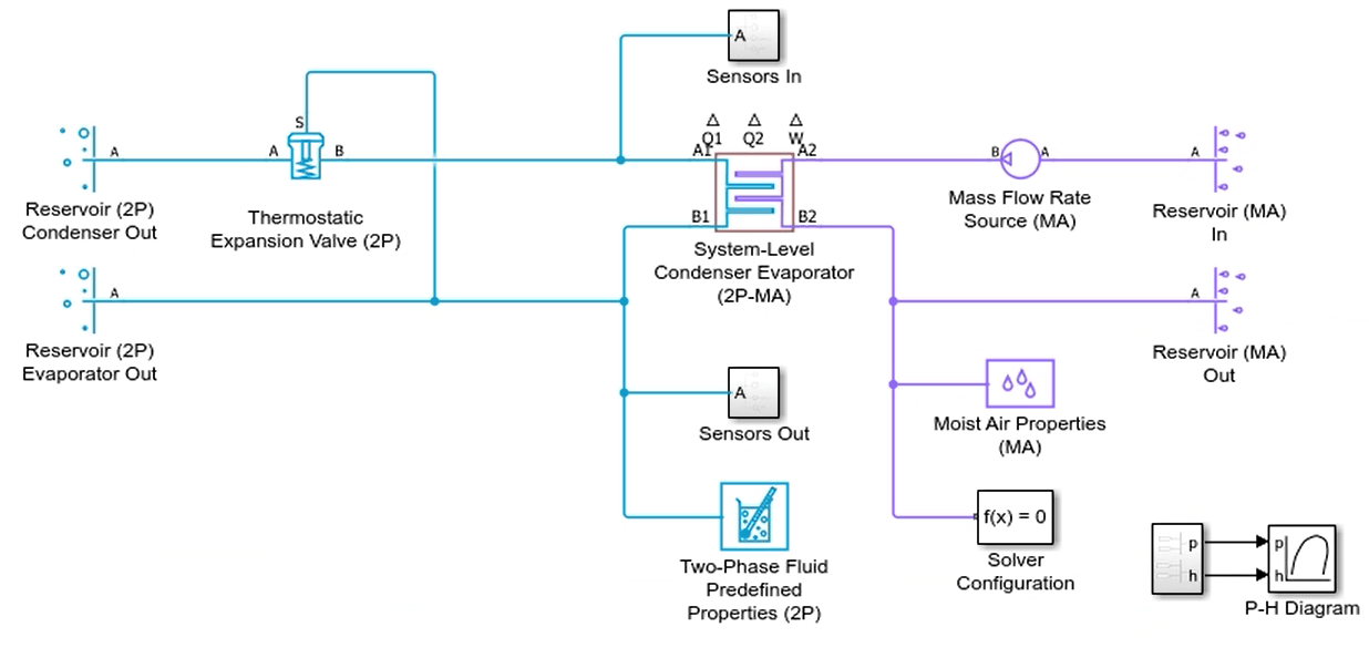
1. In the test harness from step 2, replace the Flow Rate Source (2P) block with the Thermostatic Expansion Valve (2P) block.

   1. Connect sensing port S to the evaporator outlet. This port measures the evaporator superheat.

   2. Use the refrigeration cycle data from step 1 to change the conditions in the Reservoir (2P) block upstream of the valve from the evaporator inlet conditions to match the condenser outlet conditions.

2. Set the Thermostatic Expansion Valve (2P) parameters based on the refrigeration cycle data from steps 1 and 2.

3. Run the model and use the Simscape Results Explorer to check the results. Compare your results to the previous simulation. Check that the opening fraction for your model meets the design requirements. In this example, the steady-state value of the opening_area_fraction plot is close to 0.7.

To view the example model created in this step, enter:

ModelARefrigerationCycleStep3

Step 4: Set Up the Condenser Test Harness

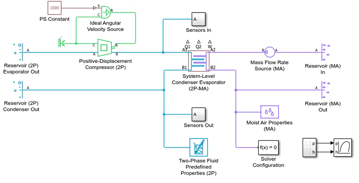
Next, build the condenser test harness using the same approach as the evaporator test harness in step 2. Unlike the mass flow rate sources, this compressor must do work on the flow.

1. Model the condenser, flow, and environmental conditions. Use a System-Level Condenser Evaporator (2P-MA) to represent a condenser that rejects heat to the outdoor environment.

2. Connect a Positive-Displacement Compressor (2P) block to drive the refrigerant flow through the condenser.

To simplify initial parameterization, you can use a Flow Rate Source (2P) block and set the Power added parameter to Isentropic to represent the compressor. Switch to the Positive-Displacement Compressor (2P) block before closing the loop in step 6, because a compressor provides more stability to the closed-loop system. This is because the flow rate varies in response to the pressure difference between the high-pressure line and the low-pressure line. In contrast, a mass flow rate source produces an idealized constant mass flow rate regardless of fluctuations in operating conditions.

3. Specify the parameters for the nominal operating condition parameters in the System-Level Condenser Evaporator (2P-MA) block.

4. Use Reservoir (MA) blocks to set up boundary conditions for the external environment. Set the air flow rate with Flow Rate Source (MA) block.

5. Use the refrigeration cycle data from step 1 to specify the Positive-Displacement Compressor (2P) block parameters. Set the Displacement specification parameter to Nominal mass flow rate and shaft speed. Then, use the value that you chose in step 2 for the Nominal mass flow rate parameter. The example model uses 0.1 kg/s. In a refrigeration cycle, the compressor drives the refrigerant flow leaving the evaporator and sends it to the condenser. As the compressor does work on the flow, it increases the thermal load on the condenser. Because this portion of the model includes the compressor, you can use the Positive-Displacement Compressor (2P) block instead of the Flow Rate Source (2P) block from step 2.

6. Run the model and use the Simscape Results Explorer to check the results. Check the temperatures of the Thermodynamic Properties Sensor (2P) blocks at the condenser inlet and evaporator outlet. Because the compressor does work on the refrigerant, the inlet temperature must be higher than the outlet.

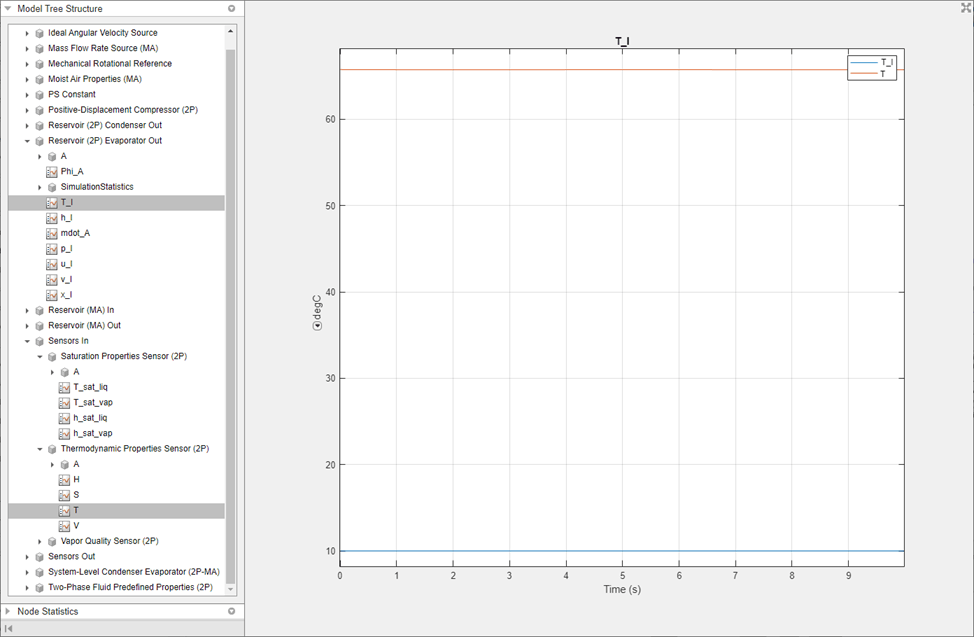
Adjust the Nominal inlet temperature parameter in the System-Level Condenser Evaporator (2P-MA) block. The condenser inlet and outlet specific enthalpy values must match the specific enthalpy end points of the high and low pressure lines in the cycle on the P-h diagram. The boundary conditions in the reservoir match the nominal operating conditions in the System-Level Heat Exchanger (2P-MA) block and the initial conditions of the System-Level Heat Exchanger (2P-MA) are the same as the nominal operating conditions, which ensures that the test harness model should be close to steady state.

7. Check that the rate of heat transfer in the condenser is approximately equal to the combined rate of heat transfer in the evaporator from step 3 and the fluid power in the compressor. Setting this value correctly helps ensure that the closed-loop system has negligible net energy transfer, which prevents pressure divergence.

8. Adjust the air mass flow rate on both the Flow Rate Source (MA) block and the System-Level Condenser Evaporator (2P-MA) block parameters to safely reject heat from the condenser. As in step 2, use the equation $$Q=\underset{}{\overset{\dot{}}{m}}{C}_p\Delta T$$ to solve for the mass flow rate. First, calculate the heat transfer using the refrigerant mass flow rate, $$Q=\underset{}{\overset{\dot{}}{m}}(h_2-h_3)$$, so Q = 0.1 kg/s * (457 kJ/kg - 267 kJ/kg) = 19 kW. Next, solve for the mass flow rate assuming an air temperature rise of about 10 °C across the condenser, from 30 °C to 40 °C: 19 kW / 1 kg/kJ/K / 10 K = 1.9 kg/s. To calculate the volumetric flow rate, divide the mass flow rate of the air by the density of air, which gives 1.9 kg/s / 1.2 kg/m = 1.58 m$${}^3$$/s.

To view the example model created in this step, enter:

ModelARefrigerationCycleStep4

Step 5: Create a Model of the Open-Loop System

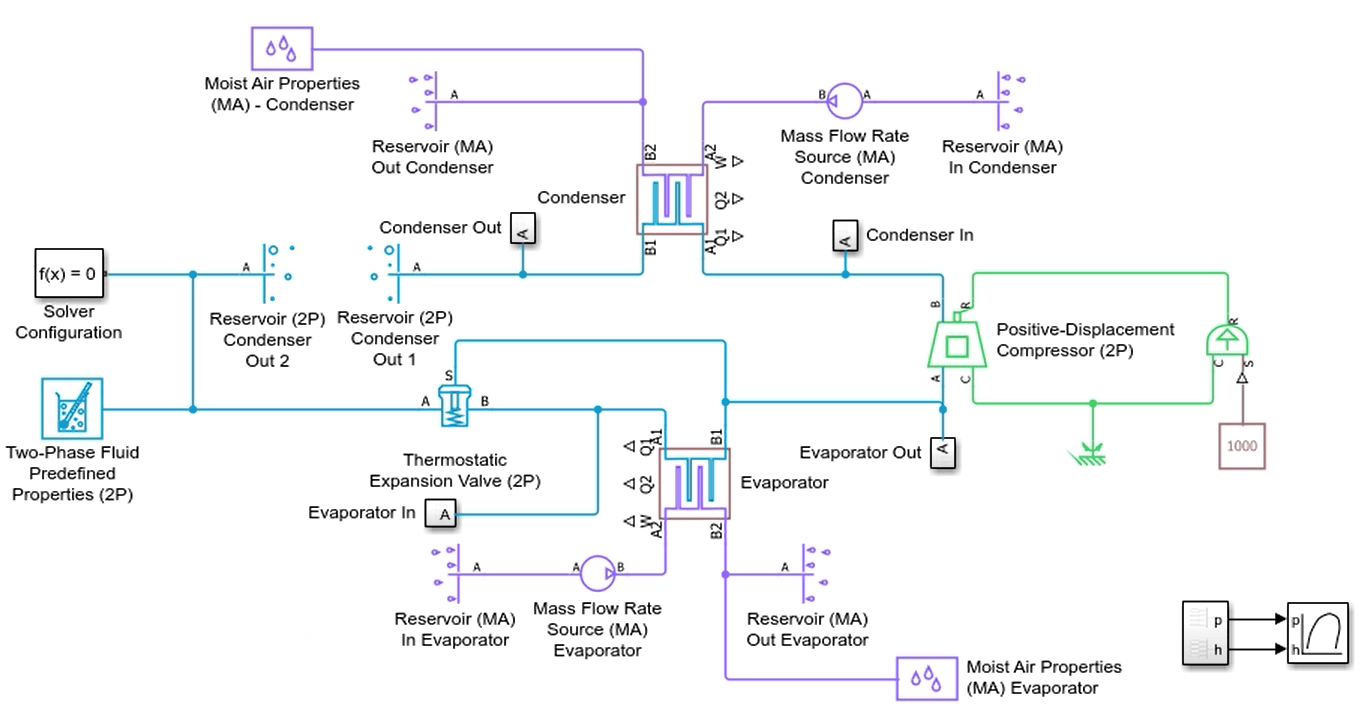
Combine the test harness models to make a model of the open-loop system.

1. Create a model with all of the components in the system:

   1. Connect the evaporator outlet from step 3 to the compressor inlet from step 4.

   2. Keep the Reservoir (2P) blocks that are connected to the condenser outlet and Thermostatic Expansion Valve (2P) block inlet. The reservoirs keep the blocks disconnected so that the model remains an open loop.

2. Run the model and use Simscape Results Explorer to check that the results are close to the results from the previous simulation.

To view the example model created in this step, enter:

ModelARefrigerationCycleStep5

Step 6: Close the Loop

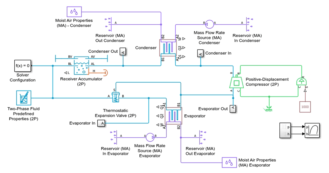
Next remove the reservoirs and connect the evaporator to the compressor to close the loop.

1. To close the loop, add a Receiver Accumulator (2P) block to the model and connect the condenser outlet to the inlet of the Thermostatic Expansion Valve (2P) block. The Receiver Accumulator (2P) block provides stability to the closed-loop system because it represents a large volume of refrigerant where the liquid level can rise and fall in response to fluctuating operating conditions. The volume depends on the size of the refrigeration system.

2. Run the model and use the Simscape Results Explorer to check that the results are close to the results from step 5.

   1. If the pressure keeps increasing or decreasing, then the condenser heat transfer might not match the combined evaporator heat transfer and compressor fluid power, which results in a net energy transfer to or from the refrigerant. Return to your harness from step 4.

   2. Check that the liquid level in the Receiver Accumulator block is stable at the steady-state nominal operating condition. Adjust its volume, if necessary.

3. Check that the refrigerant mass flow rate, evaporator pressure, and condenser pressure are stable at the steady-state nominal operating conditions.

4. Check that the liquid level in the Receiver Accumulator (2P) block is stable at the steady-state nominal operating condition and adjust its volume if it is necessary. You can use the refrigerantChargeProperties function to calculate the fluid states of any blocks that model fluid volume for a specific refrigerant charge density.

To learn more about closing the loop for systems with microchannel heat exchangers, see Considerations for Microchannel Heat Exchangers.

To view the example model created in this step, enter:

ModelARefrigerationCycleStep6

Make Additional Refinements to Fidelity

You can continue to modify and refine the design to improve the fidelity of the system model. The Refrigeration Cycle (Air Conditioning) model demonstrates a model that uses:

• A house thermal network to represent the moist air network at the evaporator

• A Fan (MA) block in place of the Flow Rate Source (MA) block

• A controller that turns the system on and off to maintain a given indoor temperature