Benchmark Solving a Linear System by Using GPU Coder

This example shows how to benchmark solving a linear system by generating CUDA® code. Use matrix left division, also known as mldivide or the backslash operator (\), to solve the system of linear equations A*x = b for x (that is, compute x = A\b).

Third-Party Prerequisites

Required

This example generates CUDA MEX and has the following third-party requirements.

• CUDA enabled NVIDIA® GPU and compatible driver.

Optional

For non-MEX builds such as static, dynamic libraries or executables, this example has the following additional requirements.

• NVIDIA toolkit.

• Environment variables for the compilers and libraries. For more information, see Third-Party Hardware and Setting Up the Prerequisite Products.

Verify GPU Environment

To verify that the compilers and libraries necessary for running this example are set up correctly, use the coder.checkGpuInstall function.

envCfg = coder.gpuEnvConfig('host');
envCfg.BasicCodegen = 1;
envCfg.Quiet = 1;
coder.checkGpuInstall(envCfg);

Determine the Maximum Data Size

Choose the appropriate matrix size for the computations by specifying the amount of system memory in GB available to the CPU and the GPU. The default value is based only on the amount of memory available on the GPU. You can specify a value that is appropriate for your system.

g = gpuDevice; 
maxMemory = 0.1*g.AvailableMemory/1024^3;

Note:

This example uses cuSOLVER libraries that have significant GPU memory requirements for creating workspaces. If you run into CUDA out-of-memory errors, reduce the maxMemory or the matrix step sizes in sizeSingle and sizeDouble.

The Benchmarking Function

This example benchmarks matrix left division (\) including the cost of transferring data between the CPU and GPU, to get a clear view of the total application time when using GPU Coder™. The application time profiling must not include the time to create sample input data. The genData.m function separates generation of test data from the entry-point function that solves the linear system.

type getData.m

function [A, b] = getData(n, clz)

%   Copyright 2017-2022 The MathWorks, Inc.

    fprintf('Creating a matrix of size %d-by-%d.\n', n, n);
    A = rand(n, n, clz) + 100*eye(n, n, clz);
    b = rand(n, 1, clz);
end

The Backslash Entry-Point Function

The backslash.m entry-point function encapsulates the (\) operation for which you want to generate code.

type backslash.m

function [x] = backslash(A,b)
%#codegen

%   Copyright 2017-2022 The MathWorks, Inc.

    coder.gpu.kernelfun();
    x = A\b;
end

Generate the GPU Code

Create a function to generate the GPU MEX function based on the particular input data size.

type genGpuCode.m

function [] = genGpuCode(A, b)

%   Copyright 2017-2022 The MathWorks, Inc.

    cfg = coder.gpuConfig('mex');
    evalc('codegen -config cfg -args {A,b} backslash');
end

Choose a Problem Size

The performance of the parallel algorithms that solve a linear system depends greatly on the matrix size. This example compares the performance of the algorithm for different matrix sizes (multiples of 1024).

sizeLimit = inf;
if ispc
    sizeLimit = double(intmax('int32'));
end
maxSizeSingle = min(floor(sqrt(maxMemory*1024^3/4)),floor(sqrt(sizeLimit/4)));
maxSizeDouble = min(floor(sqrt(maxMemory*1024^3/8)),floor(sqrt(sizeLimit/8)));
step = 1024;
if maxSizeDouble/step >= 10
    step = step*floor(maxSizeDouble/(5*step));
end
sizeSingle = 1024:step:maxSizeSingle;
sizeDouble = 1024:step:maxSizeDouble;
numReps = 5;

Compare Performance: Speedup

Use the total elapsed time as a measure of performance because that enables you to compare the performance of the algorithm for different matrix sizes. Given a matrix size, the benchmarking function creates the matrix A and the right-side b once, and then solves A\b a few times to get an accurate measure of the time it takes.

type benchFcnMat.m

function time = benchFcnMat(A, b, reps)

%   Copyright 2017-2022 The MathWorks, Inc.

    time = inf;
    % Solve the linear system a few times and take the best run
    for itr = 1:reps
        tic;
        matX = backslash(A, b);
        tcurr = toc;
        time = min(tcurr, time);
    end
end

Create a different function for GPU code execution that invokes the generated GPU MEX function.

type benchFcnGpu.m

function time = benchFcnGpu(A, b, reps)

%   Copyright 2017-2022 The MathWorks, Inc.

    time = inf;
    gpuX = backslash_mex(A, b);
    for itr = 1:reps
        tic;
        gpuX = backslash_mex(A, b);
        tcurr = toc;
        time = min(tcurr, time);
    end
end

Execute the Benchmarks

When you execute the benchmarks, the computations can take a long time to complete. Print some intermediate status information as you complete the benchmarking for each matrix size. Encapsulate the loop over all the matrix sizes in a function to benchmark single- and double-precision computations.

Actual execution times can vary across different hardware configurations. This benchmarking was done by using MATLAB R2022a on a machine with a 6 core, 3.5GHz Intel® Xeon® CPU and an NVIDIA TITAN Xp GPU.

type executeBenchmarks.m

function [timeCPU, timeGPU] = executeBenchmarks(clz, sizes, reps)

%   Copyright 2017-2022 The MathWorks, Inc.

    fprintf(['Starting benchmarks with %d different %s-precision ' ...
         'matrices of sizes\nranging from %d-by-%d to %d-by-%d.\n'], ...
            length(sizes), clz, sizes(1), sizes(1), sizes(end), ...
            sizes(end));
    timeGPU = zeros(size(sizes));
    timeCPU = zeros(size(sizes));   
    for i = 1:length(sizes)
        n = sizes(i);
        fprintf('Size : %d\n', n);
        [A, b] = getData(n, clz);
        genGpuCode(A, b);
        timeCPU(i) = benchFcnMat(A, b, reps);
        fprintf('Time on CPU: %f sec\n', timeCPU(i));
        timeGPU(i) = benchFcnGpu(A, b, reps);
        fprintf('Time on GPU: %f sec\n', timeGPU(i));
        fprintf('\n');
    end
end

Execute the benchmarks in single and double precision.

[cpu, gpu] = executeBenchmarks('single', sizeSingle, numReps);

Starting benchmarks with 8 different single-precision matrices of sizes
ranging from 1024-by-1024 to 22528-by-22528.
Size : 1024
Creating a matrix of size 1024-by-1024.
Time on CPU: 0.011866 sec
Time on GPU: 0.004042 sec

Size : 4096
Creating a matrix of size 4096-by-4096.
Time on CPU: 0.246468 sec
Time on GPU: 0.023765 sec

Size : 7168
Creating a matrix of size 7168-by-7168.
Time on CPU: 0.897369 sec
Time on GPU: 0.064114 sec

Size : 10240
Creating a matrix of size 10240-by-10240.
Time on CPU: 2.199820 sec
Time on GPU: 0.138756 sec

Size : 13312
Creating a matrix of size 13312-by-13312.
Time on CPU: 4.589138 sec
Time on GPU: 0.253298 sec

Size : 16384
Creating a matrix of size 16384-by-16384.
Time on CPU: 8.026105 sec
Time on GPU: 0.418530 sec

Size : 19456
Creating a matrix of size 19456-by-19456.
Time on CPU: 12.909238 sec
Time on GPU: 0.640920 sec

Size : 22528
Creating a matrix of size 22528-by-22528.
Time on CPU: 19.308684 sec
Time on GPU: 0.935741 sec

results.sizeSingle = sizeSingle;
results.timeSingleCPU = cpu;
results.timeSingleGPU = gpu;
[cpu, gpu] = executeBenchmarks('double', sizeDouble, numReps);

Starting benchmarks with 6 different double-precision matrices of sizes
ranging from 1024-by-1024 to 16384-by-16384.
Size : 1024
Creating a matrix of size 1024-by-1024.
Time on CPU: 0.024293 sec
Time on GPU: 0.010438 sec

Size : 4096
Creating a matrix of size 4096-by-4096.
Time on CPU: 0.431786 sec
Time on GPU: 0.129416 sec

Size : 7168
Creating a matrix of size 7168-by-7168.
Time on CPU: 1.684876 sec
Time on GPU: 0.559612 sec

Size : 10240
Creating a matrix of size 10240-by-10240.
Time on CPU: 4.476006 sec
Time on GPU: 1.505087 sec

Size : 13312
Creating a matrix of size 13312-by-13312.
Time on CPU: 8.845687 sec
Time on GPU: 3.188244 sec

Size : 16384
Creating a matrix of size 16384-by-16384.
Time on CPU: 17.680626 sec
Time on GPU: 5.831711 sec

results.sizeDouble = sizeDouble;
results.timeDoubleCPU = cpu;
results.timeDoubleGPU = gpu;

Plot the Performance

Plot the results and compare the performance on the CPU and the GPU for single and double precision.

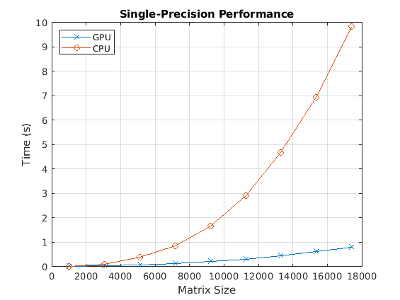
First, look at the performance of the backslash operator in single precision.

fig = figure;
ax = axes('parent', fig);
plot(ax, results.sizeSingle, results.timeSingleGPU, '-x', ...
     results.sizeSingle, results.timeSingleCPU, '-o')
grid on;
legend('GPU', 'CPU', 'Location', 'NorthWest');
title(ax, 'Single-Precision Performance')
ylabel(ax, 'Time (s)');
xlabel(ax, 'Matrix Size');

drawnow;

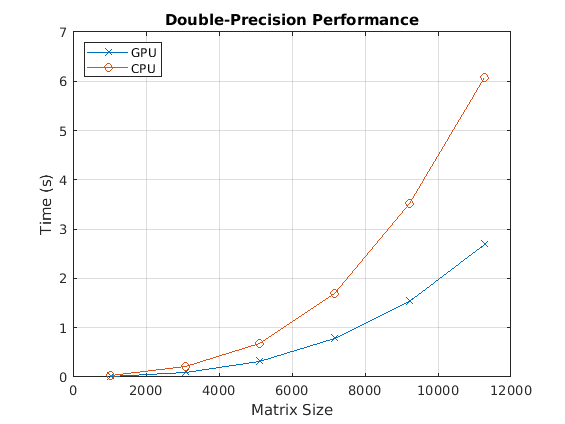
Now, look at the performance of the backslash operator in double precision.

fig = figure;
ax = axes('parent', fig);
plot(ax, results.sizeDouble, results.timeDoubleGPU, '-x', ...
     results.sizeDouble, results.timeDoubleCPU, '-o')
legend('GPU', 'CPU', 'Location', 'NorthWest');
grid on;
title(ax, 'Double-Precision Performance')
ylabel(ax, 'Time (s)');
xlabel(ax, 'Matrix Size');

drawnow;

Finally, look at the speedup of the backslash operator when comparing the GPU to the CPU.

speedupDouble = results.timeDoubleCPU./results.timeDoubleGPU;
speedupSingle = results.timeSingleCPU./results.timeSingleGPU;
fig = figure;
ax = axes('parent', fig);
plot(ax, results.sizeSingle, speedupSingle, '-v', ...
     results.sizeDouble, speedupDouble, '-*')
grid on;
legend('Single-precision', 'Double-precision', 'Location', 'SouthEast');
title(ax, 'Speedup of Computations on GPU Compared to CPU');
ylabel(ax, 'Speedup');
xlabel(ax, 'Matrix Size');

drawnow;