Implement Hardware-Efficient Hyperbolic Tangent
This example demonstrates how to compute the hyperbolic tangent of a given real-valued set of data using hardware-efficient MATLAB® code embedded in Simulink® models. The model used in this example is suitable for HDL code generation for fixed-point inputs. The algorithm employs an architecture that shares computational and memory units across different steps, which is beneficial when deploying to FPGA or ASIC devices with constrained resources. This implementation thus has a smaller throughput than a fully pipelined implementation, but it also has a smaller on-chip footprint, making it suitable for resource-conscious designs.
The Hyperbolic Tangent
The hyperbolic tangent function is the hyperbolic analogue of the circular function, and is defined as the ratio of the hyperbolic sine and hyperbolic cosine functions for a given angle .
The CORDIC Algorithm
CORDIC is an acronym for COordinate Rotation DIgital Computer, and can be used to efficiently compute many trigonometric and hyperbolic functions. For a detailed explanation of the CORDIC algorithm and its application in the calculation of a trigonometric function, see Compute Sine and Cosine Using CORDIC Rotation Kernel.
Hardware Efficient Fixed-Point Computations
The Hyperbolic Tangent HDL Optimized block supports HDL code generation for fixed-point data with binary-point scaling. It is designed with this application in mind, and employs hardware specific semantics and optimizations. One of these optimizations is resource sharing.
When deploying intricate algorithms to FPGA or ASIC devices, there is often a tradeoff between resource usage and total throughput for a given computation. Fully pipelined and parallelized algorithms have the greatest throughput, but they are often too resource intensive to deploy on real devices. By implementing scheduling logic around one or several core computational circuits, it is possible to reuse resources throughout a computation. The result is an implementation with a much smaller footprint, at the cost of a reduced total throughput. This is often an acceptable tradeoff, as resource shared designs can still meet overall latency requirements.
All of the key computational units in the Hyperbolic Tangent HDL Optimized block are reused throughout the computation lifecycle. This includes not only the CORDIC circuitry used to perform the Givens rotations, but also the adders and multipliers used for updating the angles. This saves both DSP and fabric resources when deploying to FPGA or ASIC devices.
Supported Datatypes
Single, double, binary-point scaled fixed-point, and binary-point scaled-double data types are supported for simulation. However, only binary-point scaled fixed-point data types are supported for HDL code generation.
Interfacing with the Hyperbolic Tangent HDL Optimized Block
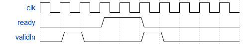
The Hyperbolic Tangent HDL Optimized block accepts data when the ready output is high, indicating that the block is ready to begin a new computation. To send input data to the block, the validIn signal must be asserted. If the block successfully registers the input value it will de-assert the ready signal, and the user must then wait until the signal is asserted again to send a new input. This protocol is summarized in the following wave diagram. Note how the first valid input to the block is discarded because the block was not ready to accept input data.
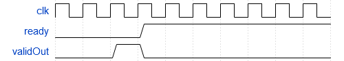
When the block has finished the computation and is ready to send the output, it will assert validOut for one clock cycle. Then ready will be asserted, indicating that the block is ready to accept a new input value.
Simulate the Example Model
Open the example model by entering at the command line:
mdl = 'fxpdemo_tanh';
open_system(mdl)
The model contains the Hyperbolic Tangent HDL Optimized block connected to a data source which takes in an array of inputs and passes an input value from the array to the Hyperbolic Tangent HDL Optimized block when it is ready to accept a new input. The output computed for each value is stored in a workspace variable. The simulation terminates when all inputs have been processed.
Define an array of inputs, tanhInput. For this example, inputs are doubles.
tanhInput = -10:0.05:10;
Simulate the model.
sim(mdl);
When the simulation is complete, a new workspace variable, tanhOutput, is created to hold the computed value for each input.
Plot the Output
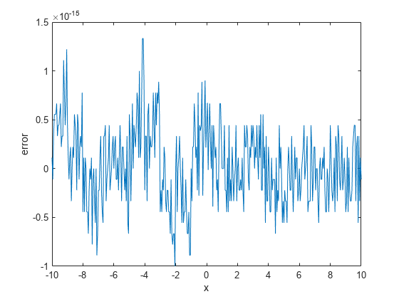
Plot the error of the calculation by comparing the output of the Hyperbolic Tangent HDL Optimized block to that of the MATLAB tanh function.
figure(1);
plot(tanhInput, tanhOutput - tanh(tanhInput'));
xlabel('x');
ylabel('error');
See Also
Hyperbolic Tangent HDL Optimized