Use Hodrick-Prescott Filter to Reproduce Original Result
This example shows how to use the Hodrick-Prescott filter to decompose a time series.
The Hodrick-Prescott filter specialized filter for trend and business cycle estimation. The filter separates a time series into trend and cyclical components (no seasonal components), the latter of which is often of interest to business cycle analysts.
Suppose a time series can be additively decomposed into a trend and business cycle component , such that, for ,
The objective function for the filter is
The programming problem is to minimize the objective over all trends components . The hyperparameter is a nonnegative smoothing parameter that penalizes the objective for large second-order differences of the trend component.
The conceptual basis for this programming problem is that the first sum minimizes the difference between the data and its trend component (which is the cyclical component) and the second sum minimizes the second-order difference of the trend component, which is analogous to minimization of the second derivative of the trend component. The programming problem is equivalent to that of a cubic spline smoother.
Use Hodrick-Prescott Filter to Analyze GNP Cyclicality
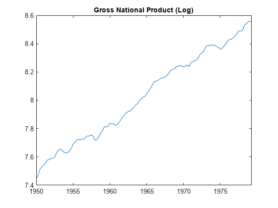
Using data similar to the data found in Hodrick and Prescott [1], plot the cyclical component of GNP. This result should coincide with the results in the paper. However, since the GNP data here and in the paper are both adjusted for seasonal variations with conversion from nominal to real values, differences can be expected due to differences in the sources for the pair of adjustments. Note that our data comes from the St. Louis Federal Reserve FRED database [2], which was downloaded with the Datafeed Toolbox™.
load Data_GNP

% Change the following two lines to try alternative periods
startdate = datetime(1950,1,1);
enddate = datetime(1979,4,1);
DTT = DataTimeTable(startdate:enddate,:);

DTT.GNPRLog = log(DTT.GNPR);
figure
plot(DTT.Time,DTT.GNPRLog)
title("Gross National Product (Log)")

Filter the series for each smoothing parameter value = 400, 1600, 6400, and . The infinite smoothing parameter detrends the data.
[TTbl4,CTbl4] = hpfilter(DTT,Smoothing=400,DataVariables="GNPRLog");
[TTbl16,CTbl16] = hpfilter(DTT,Smoothing=1600,DataVariables="GNPRLog");
[TTbl64,CTbl64] = hpfilter(DTT,Smoothing=6400,DataVariables="GNPRLog");
[TTblInf,CTblInf] = hpfilter(DTT,Smoothing=Inf,DataVariables="GNPRLog");
Plot Cyclical GNP and Its Relationship With Long-Term Trend
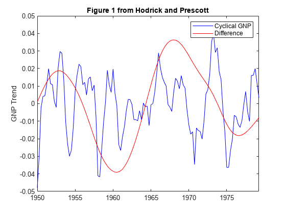
Generate Figure 1 from Hodrick and Prescott [1] by setting the slider interactive control for to 1600.
lambda =1600; [~,CTbl] = hpfilter(DTT,Smoothing=lambda,DataVariables="GNPRLog"); plot(DTT.Time,CTbl.GNPRLog,"b"); hold on plot(DTT.Time,CTblInf.GNPRLog - CTbl.GNPRLog,"r"); title("Figure 1 from Hodrick and Prescott"); ylabel("GNP Trend"); legend(["Cyclical GNP" "Difference"]); hold off

The blue line is the cyclical component with smoothing parameter 1600 and the red line is the difference with respect to the detrended cyclical component. The difference is smooth enough to suggest that the choice of smoothing parameter is appropriate.
You can use the slider control to tune the filter interactively.
Statistical Tests on Cyclical GNP
Reconstruct Table 1 from Hodrick and Prescott [1]. With the cyclical components, compute standard deviations, autocorrelations for lags 1 to 10, and perform a Dickey-Fuller unit root test to assess non-stationarity.
ACFTbl4 = autocorr(CTbl4,NumLags=10,DataVariable="GNPRLog");
ACFTbl16 = autocorr(CTbl16,NumLags=10,DataVariable="GNPRLog");
ACFTbl64 = autocorr(CTbl64,NumLags=10,DataVariable="GNPRLog");
ACFTblInf = autocorr(CTblInf,NumLags=10,DataVariable="GNPRLog");

[StatTbl4] = adftest(CTbl4,Model="ARD");
[StatTbl16] = adftest(CTbl16,Model="ARD");
[StatTbl64] = adftest(CTbl64,Model="ARD");
[StatTblInf] = adftest(CTblInf,Model="ARD");

displayResults(CTbl4,CTbl16,CTbl64,CTblInf, ...
    ACFTbl4,ACFTbl16,ACFTbl64,ACFTblInf, ...
    StatTbl4,StatTbl16,StatTbl64,StatTblInf);
Table 1 from Hodrick and Prescott Reference
              Smoothing Parameter
                     400        1600        6400    Infinity
  Std. Dev.         1.52        1.75        2.06        3.11
  Autocorrelations
           1        0.74        0.78        0.82        0.92
           2        0.38        0.47        0.57        0.81
           3        0.05        0.17        0.33        0.70
           4       -0.21       -0.07        0.12        0.59
           5       -0.36       -0.24       -0.03        0.50
           6       -0.39       -0.30       -0.10        0.44
           7       -0.35       -0.31       -0.13        0.39
           8       -0.28       -0.29       -0.15        0.35
           9       -0.22       -0.26       -0.15        0.31
          10       -0.19       -0.25       -0.17        0.26
  Unit Root        -4.35       -4.13       -3.79       -2.28
  Reject H0            1           1           1           0
As shown in [1], as increases, standard deviations increase, autocorrelations increase over longer lags, and the unit root hypothesis is rejected for all but the detrended case. These results imply that any of the cyclical series with finite smoothing is effectively stationary.
Local Function
function displayResults(gnpcycle4,gnpcycle16,gnpcycle64,gnpcycleinf,...
    gnpacf4,gnpacf16,gnpacf64,gnpacfinf,...
    gnptest4,gnptest16,gnptest64,gnptestinf)
% DISPLAYRESULTS Display cyclical GNP test results in tabular form
    fprintf(1,"Table 1 from Hodrick and Prescott Reference\n");
    fprintf(1,"  %10s  %s\n"," ","Smoothing Parameter");
    fprintf(1,"  %10s  %10s  %10s  %10s  %10s\n"," ","400","1600","6400","Infinity");
    fprintf(1,"  %-10s  %10.2f  %10.2f  %10.2f  %10.2f\n","Std. Dev.", ...
	100*std(gnpcycle4.GNPRLog),100*std(gnpcycle16.GNPRLog), ...
    100*std(gnpcycle64.GNPRLog),100*std(gnpcycleinf.GNPRLog));
    fprintf(1,"  Autocorrelations\n");
    for i = 2:11
	fprintf(1,"  %10g  %10.2f  %10.2f  %10.2f  %10.2f\n",(i-1), ...
		gnpacf4.ACF(i),gnpacf16.ACF(i),gnpacf64.ACF(i),gnpacfinf.ACF(i))
    end
    fprintf(1,"  %-10s  %10.2f  %10.2f  %10.2f  %10.2f\n","Unit Root", ...
	gnptest4.stat,gnptest16.stat,gnptest64.stat,gnptestinf.stat);
    fprintf(1,"  %-10s  %10d  %10d  %10d  %10d\n","Reject H0",...
        gnptest4.h,gnptest16.h,gnptest64.h,gnptestinf.h);
end
References
[1] Hodrick, Robert J., and Edward C. Prescott. "Postwar U.S. Business Cycles: An Empirical Investigation." Journal of Money, Credit and Banking 29, no. 1 (February 1997): 1–16. https://doi.org/10.2307/2953682.
[2] U.S. Federal Reserve Economic Data (FRED), Federal Reserve Bank of St. Louis, https://fred.stlouisfed.org/.
See Also
Topics
- When to Use the Hodrick-Prescott Filter
- Compare One-Sided and Two-Sided Hodrick-Prescott Filter Results
- Choose Time Series Filter for Business Cycle Analysis
- Compare Hodrick-Prescott Filter Formulations
- Estimate Moving Average Trend Using Moving Average Filter
- Decompose Time Series Into Additive Trend Components
- Seasonal Filters