Time Series Regression III: Influential Observations
This example shows how to detect influential observations in time series data and accommodate their effect on multiple linear regression models. It is the third in a series of examples on time series regression, following the presentation in previous examples.
Introduction
When considering the empirical limitations that affect OLS estimates, Belsley et al. [1] advise that collinearities be addressed first. A next step is to look for influential observations, whose presence, individually or in groups, have measurable effects on regression results. We distinguish the essentially metric notion of "influential observation" from the more subjective notion of "outlier," which may include any data that do not follow expected patterns.
We begin by loading relevant data from the previous example Time Series Regression II: Collinearity and Estimator Variance, and continue the analysis of the credit default model presented there:
load Data_TSReg2
dt = datetime(dateNums,'ConvertFrom','datenum','Format','yyyy');
Influential Observations
Influential observations arise in two fundamentally distinct ways. First, they may be the result of measurement or recording errors. In that case, they are just bad data, detrimental to model estimation. On the other hand, they may reflect the true distribution of the innovations process, exhibiting heteroscedasticity, skewness, or leptokurtosis for which the model fails to account. Such observations may contain abnormal sample information that is nevertheless essential to accurate model estimation. Determining the type of influential observation is difficult when looking at data alone. The best clues are often found in the data-model interactions that produce the residual series. We investigate these further in the example Time Series Regression VI: Residual Diagnostics.
Preprocessing influential observations has three components: identification, influence assessment, and accommodation. In econometric settings, identification and influence assessment are usually based on regression statistics. Accommodation, if there is any, is usually a choice between deleting data, which requires making assumptions about the DGP, or else implementing a suitably robust estimation procedure, with the potential to obscure abnormal, but possibly important, information.
Time series data differ from cross-sectional data in that deleting observations leaves "holes" in the time base of the sample. Standard methods for imputing replacement values, such as smoothing, violate the CLM assumption of strict exogeneity. If time series data exhibit serial correlation, as they often do in economic settings, deleting observations will alter estimated autocorrelations. The ability to diagnose departures from model specification, through residual analysis, is compromised. As a result, the modeling process must cycle between diagnostics and respecification until acceptable coefficient estimates produce an acceptable series of residuals.
Deletion Diagnostics
The function fitlm computes many of the standard regression statistics used to measure the influence of individual observations. These are based on a sequence of one-at-a-time row deletions of jointly observed predictor and response values. Regression statistics are computed for each delete-1 data set and compared to the statistics for the full data set.
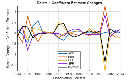
Significant changes in the coefficient estimates after deleting an observation are the main concern. The fitted model property Diagnostics.Dfbetas scales these differences by estimates of the individual coefficient variances, for comparison:
dfBetas = M0.Diagnostics.Dfbetas;

figure
hold on
plot(dt,dfBetas(:,2:end),'LineWidth',2)
plot(dt,dfBetas(:,1),'k','LineWidth',2)
hold off
legend([predNames0,'Intercept'],'Location','Best')
xlabel('Observation Deleted')
ylabel('Scaled Change in Coefficient Estimate')
title('{\bf Delete-1 Coefficient Estimate Changes}')
axis tight
grid on
Effects of the deletions on component pairs in are made apparent in a matrix of 2-D scatter plots of the changes:
figure
gplotmatrix(dfBetas,[],[],[],'o',2,[],...
            'Variable',['Const',predNames0]);
title('{\bf Delete-1 Coefficient Estimate Changes}')
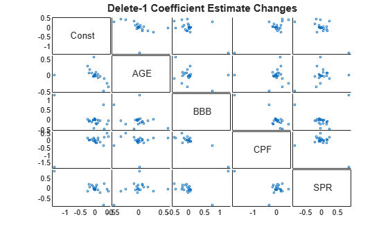
With sufficient data, these scatters tend to be approximately elliptical [2]. Outlying points can be labeled with the name of the corresponding deleted observation by typing gname(dt) at the command prompt, then clicking on a point in the plots.
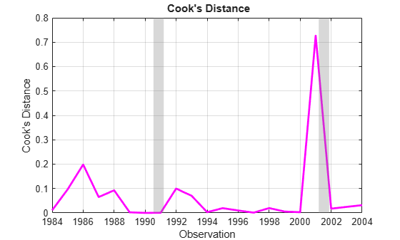
Alternatively, Cook's distance, found in the Diagnostics.CooksDistance property of the fitted model, is a common summary statistic for these plots, with contours forming ellipses centered around (that is, dfBeta = 0). Points far from the center in multiple plots have a large Cook's distance, indicating an influential observation:
cookD = M0.Diagnostics.CooksDistance;

figure;
plot(dt,cookD,'m','LineWidth',2)
recessionplot;
xlabel('Observation');
ylabel('Cook''s Distance');
title('{\bf Cook''s Distance}');
axis('tight');
grid('on');
If is the estimated coefficient vector with the observation deleted from the data, then Cook's distance is also the Euclidean distance between
and
As a result, Cook's distance is a direct measure of the influence of an observation on fitted response values.
A related measure of influence is leverage, which uses the normal equations to write
where is the hat matrix, computed from the predictor data alone. The diagonal elements of are the leverage values, giving componentwise proportions of the observed contributing to the corresponding estimates in . The leverage values, found in the Diagnostics.Leverage property of the fitted model, emphasize different sources of influence:
leverage = M0.Diagnostics.Leverage;

figure;
plot(dt,leverage,'m','LineWidth',2)
recessionplot;
xlabel('Observation');
ylabel('Leverage');
title('{\bf Leverage}');
axis('tight');
grid('on');

Another common measure of influence, the Mahalanobis distance, is just a scaled version of the leverage. The Mahalanobis distances in X0 can be computed using d = mahal(X0,X0), in which case the leverage values are given by h = d/(T0-1)+(1/T0).
Additional diagnostic plots can be created by retrieving other statistics from the Diagnostics property of a fitted model, or by using the plotDiagnostics function.
Economic Significance
Before deleting data, some kind of economic meaning should be assigned to the influential points identified by the various measures. Cook's distance, associated with changes in the overall response, shows a sharp spike in 2001. Leverage, associated with predictor data alone, shows a sharp spike in 1988. It is also noteworthy that after the sudden increase in leverage and a period of high default rates, the predictor BBB bends upward after 1991, and the percentage of lower-grade bonds begins to trend. (See a plot of the predictors in the example Time Series Regression I: Linear Models.)
Some clues are found in the economic history of the times. 2001 was a period of recession in the U.S. economy (second vertical band in the plots above), brought on, in part, by the collapse of the speculative Internet bubble and a reduction in business investments. It was also the year of the September 11 attacks, which delivered a severe shock to the bond markets. Uncertainty, rather than quantifiable risk, characterized investment decisions for the rest of that year. The 1980s, on the other hand, saw the beginning of a long-term change in the character of the bond markets. New issues of high-yield bonds, which came to be known as "junk bonds," were used to finance many corporate restructuring projects. This segment of the bond market collapsed in 1989. Following a recession (first vertical band in the plots above) and an oil price shock in 1990-1991, the high-yield market began to grow again, and matured.
The decision to delete data ultimately depends on the purpose of the model. If the purpose is mostly explanatory, deleting accurately recorded data is inappropriate. If, however, the purpose is forecasting, then it must be asked if deleting points would create a presample that is more "typical" of the past, and so the future. The historical context of the data in 2001, for example, may lead to the conclusion that it misrepresents historical patterns, and should not be allowed to influence a forecasting model. Likewise, the history of the 1980s may lead to the conclusion that a structural change occurred in the bond markets, and data prior to 1991 should be ignored for forecasts in the new regime.
For reference, we create both of the amended data sets:
% Delete 2001:
d1 = (dt ~= '2001'); % Delete 1
datesd1 = dt(d1);
Xd1 = X0(d1,:);
yd1 = y0(d1);

% Delete dates prior to 1991, as well:
dm = (datesd1 >= '1991'); % Delete many
datesdm = datesd1(dm);
Xdm = Xd1(dm,:);
ydm = yd1(dm);
Summary
The effects of the deletions on model estimation are summarized below. Tabular arrays provide a convenient format for comparing the regression statistics across models:
Md1 = fitlm(Xd1,yd1);
Mdm = fitlm(Xdm,ydm);

% Model mean squared errors:
MSEs = table(M0.MSE,...
             Md1.MSE,...
             Mdm.MSE,...
             'VariableNames',{'Original','Delete01','Post90'},...
             'RowNames',{'MSE'})
MSEs=1×3 table
           Original     Delete01      Post90
           _________    _________    _________

    MSE    0.0058287    0.0032071    0.0023762
% Coefficient estimates:
Coeffs = table(M0.Coefficients.Estimate,...
               Md1.Coefficients.Estimate,...
               Mdm.Coefficients.Estimate,...
               'VariableNames',{'Original','Delete01','Post90'},...
               'RowNames',['Const',predNames0])
Coeffs=5×3 table
             Original      Delete01      Post90
             _________    __________    _________

    Const     -0.22741      -0.12821     -0.13529
    AGE       0.016781      0.016635     0.014107
    BBB      0.0042728     0.0017657    0.0016663
    CPF      -0.014888    -0.0098507    -0.010577
    SPR       0.045488      0.024171     0.041719
% Coefficient standard errors:
StdErrs = table(M0.Coefficients.SE,...
               Md1.Coefficients.SE,...
               Mdm.Coefficients.SE,...
               'VariableNames',{'Original','Delete01','Post90'},...
               'RowNames',['Const',predNames0])
StdErrs=5×3 table
             Original     Delete01      Post90
             _________    _________    _________

    Const     0.098565     0.077746     0.086073
    AGE      0.0091845    0.0068129     0.013024
    BBB      0.0026757    0.0020942    0.0030328
    CPF      0.0038077    0.0031273    0.0041749
    SPR       0.033996     0.025849     0.027367
The MSE improves with deletion of the point in 2001, and then again with deletion of the pre-1991 data. Deleting the point in 2001 also has the effect of tightening the standard errors on the coefficient estimates. Deleting all of the data prior to 1991, however, severely reduces the sample size, and the standard errors of several of the estimates grow larger than they were with the original data.
References
[1] Belsley, D. A., E. Kuh, and R. E. Welsh. Regression Diagnostics. New York, NY: John Wiley & Sons, Inc., 1980.
[2] Weisberg, S. Applied Linear Regression. Hoboken, NJ: John Wiley & Sons, Inc., 2005.