Scalar Quantizers and Vector Quantizers
Scalar Quantizers
Analysis and Synthesis of Speech
A speech signal is usually represented in digital format, which is a sequence of binary bits. For storage and transmission applications, it is desirable to compress a signal by representing it with as few bits as possible, while maintaining its perceptual quality. Quantization is the process of representing a signal with a reduced level of precision. If you decrease the number of bits allocated for the quantization of your speech signal, the signal is distorted and the speech quality degrades.
In narrowband digital speech compression, speech signals are sampled at a rate of 8000 samples per second. Each sample is typically represented by 8 bits. This 8-bit representation corresponds to a bit rate of 64 kbits per second. Further compression is possible at the cost of quality. Most of the current low bit rate speech coders are based on the principle of linear predictive speech coding. This topic shows you how to use the Scalar Quantizer Encoder and Scalar Quantizer Decoder blocks to implement a simple speech coder.
Open the ex_sq_example1 model.

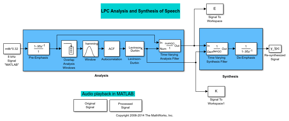
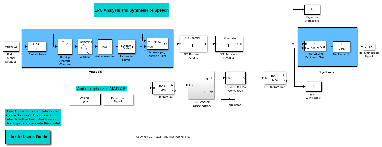
This model pre-emphasizes the input speech signal by applying an FIR filter. Then, it calculates the reflection coefficients of each frame using the Levinson-Durbin algorithm. The model uses these reflection coefficients to create the linear prediction analysis filter (lattice-structure). Next, the model calculates the residual signal by filtering each frame of the pre-emphasized speech samples using the reflection coefficients. The residual signal, which is the output of the analysis stage, usually has a lower energy than the input signal. The blocks in the synthesis stage of the model filter the residual signal using the reflection coefficients and apply an all-pole de-emphasis filter. The de-emphasis filter is the inverse of the pre-emphasis filter. The result is the full recovery of the original signal.
Run this model.
Double-click the Original Signal and Processed Signal blocks and listen to both the original and the processed signal. There is no significant difference between the two because no quantization was performed.
To better approximate a real-world speech analysis and synthesis system, quantize the residual signal and reflection coefficients before they are transmitted.
Identify Your Residual Signal and Reflection Coefficients
In the previous topic, Analysis and Synthesis of Speech, you learned the theory behind the LPC Analysis and Synthesis of Speech example model. In this topic, you define the residual signal and the reflection coefficients in your MATLAB® workspace as the variables E and K, respectively. Later, you use these values to create your scalar quantizers:
Open the
ex_sq_example1model in the Analysis and Synthesis of Speech topic.From the Simulink® Sinks library, click-and-drag two To Workspace blocks into your model.
Connect the output of the Levinson-Durbin block to one of the To Workspace blocks.
Double-click this To Workspace block and set the Variable name parameter to
K. Click OK.Connect the output of the Time-Varying Analysis Filter block to the other To Workspace block.
Double-click this To Workspace block and set the Variable name parameter to
E. Click OK.
Your model should now look similar to this figure.
Alternatively, you can open the ex_sq_example2 model.
Run your model.
The residual signal E and your reflection coefficients K are defined in the MATLAB workspace.
Add a Scalar Quantizer
In this topic, you add scalar quantizer encoders and decoders to quantize the residual signal E and the reflection coefficients K:
Open the
ex_sq_example2model in Identify Your Residual Signal and Reflection Coefficients.Run this model to define the variables E and K in the MATLAB workspace.
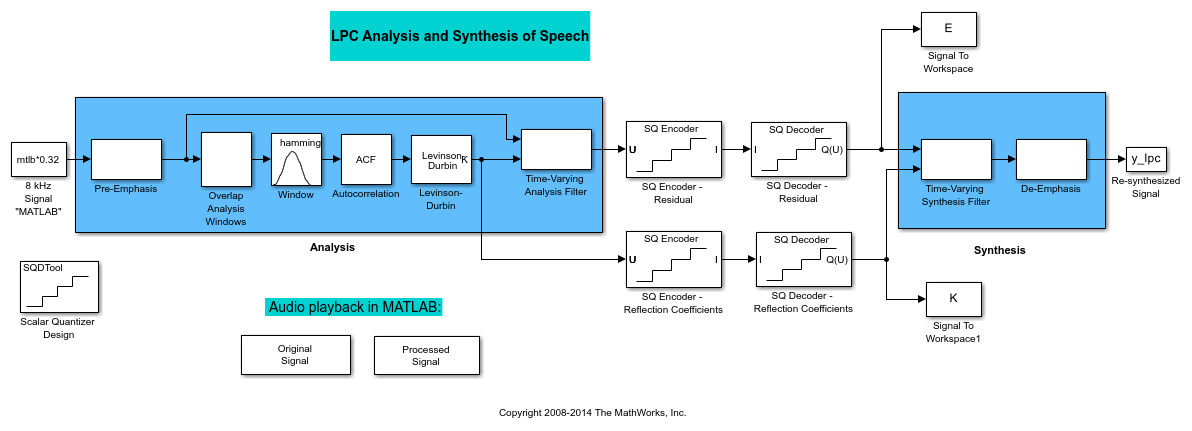
From the Quantizers library, click-and-drag a Scalar Quantizer Encoder and Scalar Quantizer Decoder blocks to the model for each signal you want to quantize. Quantize the residual signal E and the reflection coefficients K.
Your model should look similar to the following figure.
Alternatively, you can open the ex_sq_example3 model.
Run your model.
Double-click the Original Signal and Processed Signal blocks, and listen to both signals. Again, there is no perceptible difference between the two. You can therefore conclude that quantizing your residual and reflection coefficients did not affect the ability of your system to accurately reproduce the input signal.
You have now quantized the residual and reflection coefficients. The bit rate of a quantization system is calculated as (bits per frame)*(frame rate).
In this example, the bit rate is [(80 residual samples/frame)*(7 bits/sample) + (12 reflection coefficient samples/frame)*(7 bits/sample)]*(100 frames/second), or 64.4 kbits per second. This is higher than most modern speech coders, which typically have a bit rate of 8 to 24 kbits per second. If you decrease the number of bits allocated for the quantization of the reflection coefficients or the residual signal, the overall bit rate would decrease. However, the speech quality would also degrade.
For information about decreasing the bit rate without affecting speech quality, see Vector Quantizers.
Vector Quantizers
Build Your Vector Quantizer Model
In the previous section, you quantized your residual signal and reflection coefficients. The bit rate of your scalar quantization system was 64.4 kbits per second. This bit rate is higher than most modern speech coders. To accommodate a greater number of users in each channel, you need to lower this bit rate while maintaining the quality of your speech signal. You can use vector quantizers, which exploit the correlations between each sample of a signal, to accomplish this task.
In this topic, you modify your scalar quantization model so that you are using a split vector quantizer to quantize your reflection coefficients:
Open the
ex_vq_example1model. The example modelex_vq_example1adds a new LSF Vector Quantization subsystem to theex_sq_example3model. This subsystem is preconfigured to work as a vector quantizer. You can use this subsystem to encode and decode your reflection coefficients using the split vector quantization method.Delete the SQ Encoder - Reflection Coefficients and SQ Decoder - Reflection Coefficients blocks.
From the Simulink Sinks library, click-and-drag a Terminator block into your model.
From the DSP System Toolbox™ Estimation > Linear Prediction library, click-and-drag a LSF/LSP to LPC Conversion block and two LPC to/from RC blocks into your model.
Connect the blocks as shown in the following figure. You do not need to connect Terminator blocks to the P ports of the LPC to/from RC blocks. These ports disappear once you set block parameters.
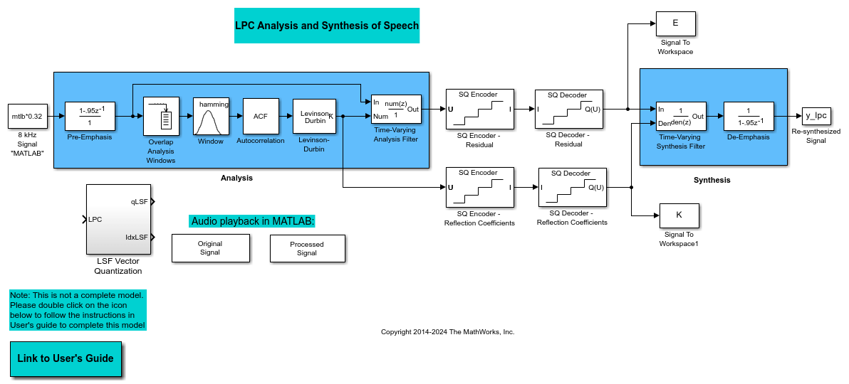
You have modified your model to include a subsystem capable of vector quantization. In the next topic, you reset your model parameters to quantize your reflection coefficients using the split vector quantization method.
Configure and Run Your Model
In the previous topic, you configured your scalar quantization model for vector quantization by adding the LSF Vector Quantization subsystem. In this topic, you set your block parameters and quantize your reflection coefficients using the split vector quantization method.
If the model you created in Build Your Vector Quantizer Model is not open on your desktop, open an equivalent model, ex_vq_example2.
Double-click the LSF Vector Quantization subsystem, and then double-click the LSF Split VQ subsystem. The subsystem opens, and you see the three Vector Quantizer Encoder blocks used to implement the split vector quantization method.
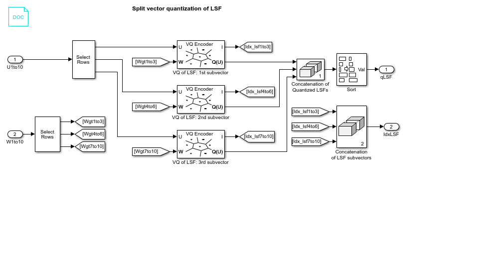
This subsystem divides each vector of 10 line spectral frequencies (LSFs), which represent your reflection coefficients, into three LSF subvectors. Each of these subvectors is sent to a separate vector quantizer. This method is called split vector quantization.
Double-click the VQ of LSF: 1st subvector block. The Block Parameters: VQ of LSF: 1st subvector dialog box opens.
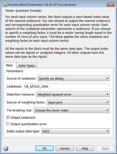
The variable CB_lsf1to3_10bit is the codebook for the subvector that contains the first three elements of the LSF vector. It is a 3-by-1024 matrix, where 3 is the number of elements in each codeword and 1024 is the number of codewords in the codebook. Because  , it takes 10 bits to quantize this first subvector. Similarly, a 10-bit vector quantizer is applied to the second and third subvectors, which contain elements 4 to 6 and 7 to 10 of the LSF vector, respectively. Therefore, it takes 30 bits to quantize all three subvectors.
Note: If you used the vector quantization method to quantize your reflection coefficients, you would need  or 1.0737e9 codebook values to achieve the same degree of accuracy as the split vector quantization method.
In your model file, double-click the Autocorrelation block and set the Maximum non-negative lag (less than input length) parameter to 10. Click OK. This parameter controls the number of linear polynomial coefficients (LPCs) that are input to the split vector quantization method.
Double-click the LPC to/from RC block that is connected to the input of the LSF Vector Quantization subsystem. Clear the Output normalized prediction error power check box. Click OK. Double-click the LSF/LSP to LPC Conversion block and set the Input parameter to LSF in range (0 to pi). Click OK.
Double-click the LPC to/from RC block that is connected to the output of the LSF/LSP to LPC Conversion block. Set the Type of conversion parameter to LPC to RC, and clear the Output normalized prediction error power check box. Click OK.
Alternatively, you can open the ex_vq_example3 model.
Run your model.
Double-click the Original Signal and Processed Signal blocks to listen to both the original and the processed signal. There is no perceptible difference between the two. Quantizing your reflection coefficients using a split vector quantization method produced good quality speech without much distortion.
You have now used the split vector quantization method to quantize your reflection coefficients. The vector quantizers in the LSF Vector Quantization subsystem use 30 bits to quantize a frame containing 80 reflection coefficients. The bit rate of a quantization system is calculated as (bits per frame)*(frame rate).
In this example, the bit rate is [(80 residual samples/frame)*(7 bits/sample) + (30 bits/frame)]*(100 frames/second), or 59 kbits per second. This is less than 64.4 kbits per second, the bit rate of the scalar quantization system. However, the quality of the speech signal did not degrade. If you want to further reduce the bit rate of your system, you can use the vector quantization method to quantize the residual signal.