Train PPO Agent for Automatic Parking Valet
This example demonstrates the design of a hybrid controller for an automatic search and parking task. The hybrid controller uses model predictive control (MPC) to follow a reference path in a parking lot and a trained reinforcement learning (RL) agent to perform the parking maneuver.
The automatic parking algorithm in this example executes a series of maneuvers while simultaneously sensing and avoiding obstacles in tight spaces. It switches between an adaptive MPC controller and an RL agent to complete the parking maneuver. The MPC controller moves the vehicle at a constant speed along a reference path while an algorithm searches for an empty parking spot. When a spot is found, the RL Agent takes over and executes a pretrained parking maneuver. Prior knowledge of the environment (the parking lot) including the locations of the empty spots and parked vehicles is available to the controllers.
Fix Random Seed Generator to Improve Reproducibility
The example code may involve computation of random numbers at various stages such as initialization of the agent, creation of the actor and critic, resetting the environment during simulations, generating observations (for stochastic environments), generating exploration actions, and sampling min-batches of experiences for learning. Fixing the random number stream preserves the sequence of the random numbers every time you run the code and improves reproducibility of results. You will fix the random number stream at various locations in the example.
Fix the random number stream with the seed 0 and random number algorithm Mersenne Twister. For more information on random number generation see rng.
previousRngState = rng(0,"twister")previousRngState = struct with fields:
Type: 'twister'
Seed: 0
State: [625x1 uint32]
The output previousRngState is a structure that contains information about the previous state of the stream. You will restore the state at the end of the example.
Parking Lot
The parking lot is represented by the ParkingLot class (provided in the example folder), which stores information about the ego vehicle, empty parking spots, and static obstacles (parked cars). Each parking spot has a unique index number and an indicator light that is either green (free) or red (occupied). Parked vehicles are represented in black.
Create a ParkingLot object with a free spot at location 7.
freeSpotIdx = 7;
map = ParkingLot(freeSpotIdx);

Specify an initial pose for the ego vehicle. The target pose is determined based on the first available free spot as the vehicle navigates the parking lot.
egoInitialPose = [20, 15, 0];
Compute the target pose for the vehicle using the createTargetPose function. The target pose corresponds to the location in freeSpotIdx.
egoTargetPose = createTargetPose(map,freeSpotIdx)
egoTargetPose = 1×3

   47.7500    4.9000   -1.5708
Sensor Modules
The parking algorithm uses camera and lidar sensors to gather information from the environment.
Camera
The field of view of a camera mounted on the ego vehicle is represented by the area shaded in green in the following figure. The camera has a field of view bounded by and a maximum measurement depth of 10 m.
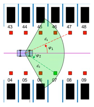
As the ego vehicle moves forward, the camera module senses the parking spots that fall within the field of view and determines whether a spot is free or occupied. For simplicity, this action is implemented using geometrical relationships between the spot locations and the current vehicle pose. A parking spot is within the camera range if and , where is the distance to the parking spot and is the angle to the parking spot.
Lidar
The reinforcement learning agent uses lidar sensor readings to determine the proximity of the ego vehicle to other vehicles in the environment. The lidar sensor in this example is also modeled using geometrical relationships. Lidar distances are measured along 12 line segments that radially emerge from the center of the ego vehicle. When a lidar line intersects an obstacle, it returns the distance of the obstacle from the vehicle. The maximum measurable lidar distance along any line segment is 6 m.

Auto Parking Valet Model
The parking valet model, including the controllers, ego vehicle, sensors, and parking lot, is implemented in Simulink®.
Load the auto parking valet parameters into the MATLAB workspace.
autoParkingValetParams
Open the Simulink model.
mdl = "rlAutoParkingValet";
open_system(mdl)
The ego vehicle dynamics in this model are represented by a single-track bicycle model with two inputs: vehicle speed (m/s) and steering angle (radians). The MPC and RL controllers are placed within Enabled Subsystem blocks that are activated by signals representing whether the vehicle has to search for an empty spot or execute a parking maneuver. The enable signals are determined by the Camera algorithm within the Vehicle Mode subsystem. Initially, the vehicle is in search mode and the MPC controller tracks the reference path. When a free spot is found, park mode is activated and the RL agent executes the parking maneuver.
Adaptive Model Predictive Controller
Create the adaptive MPC controller object for reference trajectory tracking using the createMPCForParking script (provided in the example folder). For more information see Adaptive MPC (Model Predictive Control Toolbox).
createMPCForParking
Reinforcement Learning Environment
The environment for training the RL agent is the region shaded in red in the following figure. Due to symmetry in the parking lot, training within this region is sufficient for the policy to adjust to other regions after applying appropriate coordinate transformations to the observations (these transformations are performed in the Observation and Reward group inside the RL Controller block). Using this smaller training region significantly reduces training time compared to training over the entire parking lot.

For this environment:
The training region is a 22.5 m x 20 m space with the target spot at its horizontal center.
The observations are the position errors and of the ego vehicle with respect to the target pose, the sine and cosine of the true heading angle , and the lidar sensor readings.
The vehicle speed during parking is a constant 2 m/s.
The action signals are discrete steering angles that range between +/- 45 degrees in steps of 15 degrees.
The vehicle is considered parked if the errors with respect to target pose are within specified tolerances of ±0.75 m (position) and ±10 degrees (orientation).
The episode terminates if the ego vehicle goes out of the bounds of the training region, collides with an obstacle, or parks successfully.
The reward provided at time t, is:
Here, , , and are the position and heading angle errors of the ego vehicle from the target pose, and is the steering angle. (0 or 1) indicates whether the vehicle has parked and (0 or 1) indicates if the vehicle has collided with an obstacle at time .
The coordinate transformations on vehicle pose observations for different parking spot locations are as follows:
1-14: no transformation
15-22:
23-36:
37-40:
41-52:
53-64:
Create the observation and action specifications for the environment.
numObservations = 16;
obsInfo = rlNumericSpec([numObservations 1]);
obsInfo.Name = "observations";

steerMax = pi/4;
discreteSteerAngles = -steerMax : deg2rad(15) : steerMax;
actInfo = rlFiniteSetSpec(num2cell(discreteSteerAngles));
actInfo.Name = "actions";
numActions = numel(actInfo.Elements);
Create the Simulink environment interface, specifying the path to the RL Agent block.
blk = mdl + "/RL Controller/RL Agent";
env = rlSimulinkEnv(mdl,blk,obsInfo,actInfo);
Specify a reset function for training. The autoParkingValetResetFcn function (provided at the end of this example) resets the initial pose of the ego vehicle to random values at the start of each episode.
env.ResetFcn = @autoParkingValetResetFcn;
For more information on creating Simulink environments, see rlSimulinkEnv (Reinforcement Learning Toolbox).
Create PPO Agent
You will create and train a PPO agent in this example. The agent uses:
A value function critic to estimate the value of the policy. The critic takes the current observation as input and returns a single scalar as output (the estimated discounted cumulative long-term reward for following the policy from the state corresponding to the current observation).
A stochastic actor for computing actions. This actor takes an observation as input and returns as output a random action sampled (among the finite number of possible actions) from a categorical probability distribution.
Create an agent initialization object to initialize the networks with the hidden layer size 128.
initOpts = rlAgentInitializationOptions(NumHiddenUnit=128);
Specify hyperparameters for training using the rlPPOAgentOptions (Reinforcement Learning Toolbox) object:
Specify an experience horizon of 230 steps. A large experience horizon can improve the stability of the training.
Train with
40epochs and mini-batches of length 100. Smaller mini-batches are computationally efficient but may introduce variance in training. Contrarily, larger batch sizes can make the training stable but require higher memory.Specify a learning rate of 4e-4 for the actor and 3e-5 for the critic. A large learning rate causes drastic updates which may lead to divergent behaviors, while a low value may require many updates before reaching the optimal point.
Specify an objective function clip factor of 0.2 for improving training stability.
Specify a discount factor value of 0.99 to promote long term rewards.
Specify an entropy loss weight factor of 0.01 to enhance exploration during training.
% actor and critic optimizer options
actorOpts = rlOptimizerOptions(LearnRate=4e-4, ...
    GradientThreshold=1);
criticOpts = rlOptimizerOptions(LearnRate=3e-5, ...
    GradientThreshold=1);

% agent options
agentOpts = rlPPOAgentOptions(...
    ExperienceHorizon       = 230,...
    ActorOptimizerOptions   = actorOpts,...
    CriticOptimizerOptions  = criticOpts,...
    MiniBatchSize           = 100,...
    NumEpoch                = 40,...
    SampleTime              = Ts,...
    DiscountFactor          = 0.99, ...
    ClipFactor              = 0.2, ...
    EntropyLossWeight       = 0.01);
Fix the random number stream so that the agent is always initialized with the same parameter values.
rng(0,"twister");Create the agent using the input specifications, initialization options, and the agent options objects.
agent = rlPPOAgent(obsInfo, actInfo, initOpts, agentOpts);
Train Agent
To train the PPO agent, specify the following training options.
Run the training for at most 10000 episodes, with each episode lasting at most 200 time steps.
Display the training progress in the Reinforcement Learning Training Monitor window (set the
Plotsoption) and disable the command line display (set theVerboseoption tofalse).Specify an averaging window length of 200 for the episode reward.
Evaluate the performance of the greedy policy every 20 training episodes, averaging the cumulative reward of 5 simulations.
Stop the training when the evaluation score reaches 100.
% training options
trainOpts = rlTrainingOptions(...
    MaxEpisodes=10000,...
    MaxStepsPerEpisode=200,...
    ScoreAveragingWindowLength=200,...
    Plots="training-progress",...
    Verbose=false,...
    StopTrainingCriteria="EvaluationStatistic",...
    StopTrainingValue=100);

% agent evaluation
evl = rlEvaluator(EvaluationFrequency=20, NumEpisodes=5);
Fix the random stream for reproducibility.
rng(0,"twister");Train the agent using the train (Reinforcement Learning Toolbox) function. Training this agent is a computationally intensive process that takes several minutes to complete. To save time while running this example, load a pretrained agent by setting doTraining to false. To train the agent yourself, set doTraining to true.
doTraining =false; if doTraining trainingStats = train(agent,env,trainOpts,Evaluator=evl); else load('rlAutoParkingValetAgent.mat','agent'); end

Simulate Agent
Fix the random stream for reproducibility.
rng(0,"twister");Simulate the model to park the vehicle in the parking spot specified by freeSpotIdx (1 to 64).
freeSpotIdx = 7;
sim(mdl);
7;
sim(mdl);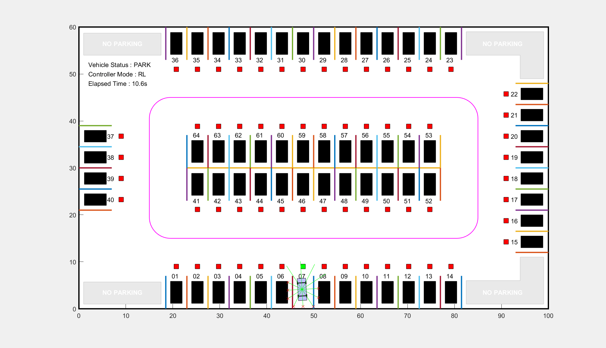
For the parking spot location 7, the vehicle reaches the target pose within the specified error tolerances of +/- 0.75 m (position) and +/-10 degrees (orientation).
To view the ego vehicle position and orientation, open the Ego Vehicle Pose scope.
open_system(mdl + "/Ego Vehicle Model/Ego Vehicle Pose");
Restore the random number stream using the information stored in previousRngState.
rng(previousRngState);
Environment Reset Function
function in = autoParkingValetResetFcn(in)
% Reset function for auto parking valet example
choice = rand;
if choice <= 0.35
    x = 37;
    y = 16;
    t = deg2rad(-45 + 2*45*rand);
elseif choice <= 0.70
    x = 58;
    y = 16;
    t = deg2rad(-225 + 2*45*rand);
else
    zone = randperm(3,1);
    switch zone
        case 1
            x = 36.5 + (45.5-36.5)*rand;
            t = deg2rad(-45 + 2*45*rand);
        case 2
            x = 45.5 + (50-45.5)*rand;
            t = deg2rad(-135 + 2*45*rand);
        case 3
            x = 50 + (59-50)*rand;
            t = deg2rad(-225 + 2*45*rand);
            if t <= -pi
                t = 2*pi + t;
            end
    end
    y = 10 + (20-10)*rand;
end
pose = [x,y,t];
speed = 5 * rand;
in = setVariable(in,'egoInitialPose',pose);
in = setVariable(in,'egoInitialSpeed',speed);
end
See Also
train (Reinforcement Learning Toolbox)
Related Topics
- Train Reinforcement Learning Agents (Reinforcement Learning Toolbox)
- Create Policies and Value Functions (Reinforcement Learning Toolbox)
You can also select a web site from the following list
Americas
- América Latina (Español)
- Canada (English)
- United States (English)
Europe
- Belgium (English)
- Denmark (English)
- Deutschland (Deutsch)
- España (Español)
- Finland (English)
- France (Français)
- Ireland (English)
- Italia (Italiano)
- Luxembourg (English)
- Netherlands (English)
- Norway (English)
- Österreich (Deutsch)
- Portugal (English)
- Sweden (English)
- Switzerland
- United Kingdom (English)
Asia Pacific
- Australia (English)
- India (English)
- New Zealand (English)
- 中国
- 日本Japanese (日本語)
- 한국Korean (한국어)