Learning Vector Quantization (LVQ) Neural Networks
Architecture
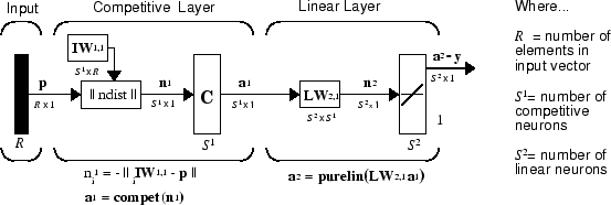
The LVQ network architecture is shown below.

An LVQ network has a first competitive layer and a second linear layer. The competitive layer learns to classify input vectors in much the same way as the competitive layers of Cluster with Self-Organizing Map Neural Network described in this topic. The linear layer transforms the competitive layer’s classes into target classifications defined by the user. The classes learned by the competitive layer are referred to as subclasses and the classes of the linear layer as target classes.
Both the competitive and linear layers have one neuron per (sub or target) class. Thus, the competitive layer can learn up to S1 subclasses. These, in turn, are combined by the linear layer to form S2 target classes. (S1 is always larger than S2.)
For example, suppose neurons 1, 2, and 3 in the competitive layer all learn subclasses of the input space that belongs to the linear layer target class 2. Then competitive neurons 1, 2, and 3 will have LW2,1 weights of 1.0 to neuron n2 in the linear layer, and weights of 0 to all other linear neurons. Thus, the linear neuron produces a 1 if any of the three competitive neurons (1, 2, or 3) wins the competition and outputs a 1. This is how the subclasses of the competitive layer are combined into target classes in the linear layer.
In short, a 1 in the ith row of a1 (the rest to the elements of a1 will be zero) effectively picks the ith column of LW2,1 as the network output. Each such column contains a single 1, corresponding to a specific class. Thus, subclass 1s from layer 1 are put into various classes by the LW2,1a1 multiplication in layer 2.
You know ahead of time what fraction of the layer 1 neurons should be classified into the various class outputs of layer 2, so you can specify the elements of LW2,1 at the start. However, you have to go through a training procedure to get the first layer to produce the correct subclass output for each vector of the training set. This training is discussed in Training. First, consider how to create the original network.
Creating an LVQ Network
You can create an LVQ network with the function lvqnet,
net = lvqnet(S1,LR,LF)
where
S1is the number of first-layer hidden neurons.LRis the learning rate (default 0.01).LFis the learning function (default islearnlv1).
Suppose you have 10 input vectors. Create a network that assigns each of these input vectors to one of four subclasses. Thus, there are four neurons in the first competitive layer. These subclasses are then assigned to one of two output classes by the two neurons in layer 2. The input vectors and targets are specified by
P = [-3 -2 -2 0 0 0 0 2 2 3; 0 1 -1 2 1 -1 -2 1 -1 0];
and
Tc = [1 1 1 2 2 2 2 1 1 1];
It might help to show the details of what you get from these two lines of code.
P,Tc
P =
    -3    -2    -2     0     0     0     0     2     2     3
     0     1    -1     2     1    -1    -2     1    -1     0
Tc =
     1     1     1     2     2     2     2     1     1     1
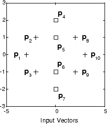
A plot of the input vectors follows.

As you can see, there are four subclasses of input vectors. You want a network that classifies p1, p2, p3, p8, p9, and p10 to produce an output of 1, and that classifies vectors p4, p5, p6, and p7 to produce an output of 2. Note that this problem is nonlinearly separable, and so cannot be solved by a perceptron, but an LVQ network has no difficulty.
Next convert the Tc matrix to target vectors.
T = ind2vec(Tc);
This gives a sparse matrix T that can be displayed in full
with
targets = full(T)
which gives
targets =
     1     1     1     0     0     0     0     1     1     1
     0     0     0     1     1     1     1     0     0     0
This looks right. It says, for instance, that if you have the first column of
P as input, you should get the first column of
targets as an output; and that output says the input falls in
class 1, which is correct. Now you are ready to call
lvqnet.
Call lvqnet to create a network with four neurons.
net = lvqnet(4);
Configure and confirm the initial values of the first-layer weight matrix are initialized by the function midpoint to values in the center of the input data range.
net = configure(net,P,T);
net.IW{1}
ans =
     0     0
     0     0
     0     0
     0     0
Confirm that the second-layer weights have 60% (6 of the 10 in
Tc) of its columns with a 1 in the first row, (corresponding
to class 1), and 40% of its columns have a 1 in the second row (corresponding to
class 2). With only four columns, the 60% and 40% actually round to 50% and there
are two 1's in each row.
net.LW{2,1}
ans =
     1     1     0     0
     0     0     1     1
This makes sense too. It says that if the competitive layer produces a 1 as the first or second element, the input vector is classified as class 1; otherwise it is a class 2.
You might notice that the first two competitive neurons are connected to the first linear neuron (with weights of 1), while the second two competitive neurons are connected to the second linear neuron. All other weights between the competitive neurons and linear neurons have values of 0. Thus, each of the two target classes (the linear neurons) is, in fact, the union of two subclasses (the competitive neurons).
You can simulate the network with sim. Use the original P matrix as input just to
see what you get.
Y = net(P);
Yc = vec2ind(Y)
Yc =
     1     1     1     1     1     1     1     1     1     1
The network classifies all inputs into class 1. Because this is not what you want, you have to train the network (adjusting the weights of layer 1 only), before you can expect a good result. The next two sections discuss two LVQ learning rules and the training process.
LVQ1 Learning Rule (learnlv1)
LVQ learning in the competitive layer is based on a set of input/target pairs.
Each target vector has a single 1. The rest of its elements are 0. The 1 tells the proper classification of the associated input. For instance, consider the following training pair.
Here there are input vectors of three elements, and each input vector is to be assigned to one of four classes. The network is to be trained so that it classifies the input vector shown above into the third of four classes.
To train the network, an input vector p is
presented, and the distance from p to each row of
the input weight matrix IW1,1 is computed with the function
negdist. The hidden neurons of layer
1 compete. Suppose that the ith element of n1 is most positive, and neuron
i* wins the competition. Then the competitive transfer
function produces a 1 as the i*th element of a1. All other elements of
a1 are 0.
When a1 is multiplied by the layer 2 weights LW2,1, the single 1 in a1 selects the class k* associated with the input. Thus, the network has assigned the input vector p to class k* and α2k* will be 1. Of course, this assignment can be a good one or a bad one, for tk* can be 1 or 0, depending on whether the input belonged to class k* or not.
Adjust the i*th row of IW1,1 in such a way as to move this row closer to the input vector p if the assignment is correct, and to move the row away from p if the assignment is incorrect. If p is classified correctly,
compute the new value of the i*th row of IW1,1 as
On the other hand, if p is classified incorrectly,
compute the new value of the i*th row of IW1,1 as
You can make these corrections to the i*th row of IW1,1 automatically, without affecting other rows of IW1,1, by back-propagating the output errors to layer 1.
Such corrections move the hidden neuron toward vectors that fall into the class for which it forms a subclass, and away from vectors that fall into other classes.
The learning function that implements these changes in the layer 1 weights in LVQ
networks is learnlv1. It can be applied during
training.
Training
Next you need to train the network to obtain first-layer weights that lead to the
correct classification of input vectors. You do this with train as with the following commands. First, set the training epochs
to 150. Then, use train:
net.trainParam.epochs = 150;
net = train(net,P,T);
Now confirm the first-layer weights.
net.IW{1,1}
ans =
    0.3283    0.0051
   -0.1366    0.0001
   -0.0263    0.2234
         0   -0.0685
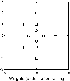
The following plot shows that these weights have moved toward their respective classification groups.

To confirm that these weights do indeed lead to the correct classification, take
the matrix P as input and simulate the network. Then see what
classifications are produced by the network.
Y = net(P);
Yc = vec2ind(Y)
This gives
Yc =
     1     1     1     2     2     2     2     1     1     1
which is expected. As a last check, try an input close to a vector that was used in training.
pchk1 = [0; 0.5];
Y = net(pchk1);
Yc1 = vec2ind(Y)
This gives
Yc1 =
     2
This looks right, because pchk1 is close to other vectors
classified as 2. Similarly,
pchk2 = [1; 0];
Y = net(pchk2);
Yc2 = vec2ind(Y)
gives
Yc2 =
     1
This looks right too, because pchk2 is close to other vectors
classified as 1.
You might want to try the example program Learning Vector Quantization. It follows the discussion of training given above.
Supplemental LVQ2.1 Learning Rule (learnlv2)
The following learning rule is one that might be applied
after first applying LVQ1. It can improve the result of the
first learning. This particular version of LVQ2 (referred to as LVQ2.1 in the
literature [Koho97]) is embodied in
the function learnlv2. Note again that LVQ2.1 is
to be used only after LVQ1 has been applied.
Learning here is similar to that in learnlv2 except now two vectors of layer 1 that are closest to the
input vector can be updated, provided that one belongs to the correct class and one
belongs to a wrong class, and further provided that the input falls into a
“window” near the midplane of the two vectors.
The window is defined by
where
(where di and dj are the Euclidean distances of p from i*IW1,1 and j*IW1,1, respectively). Take a value for w in the range 0.2 to 0.3. If you pick, for instance, 0.25, then s = 0.6. This means that if the minimum of the two distance ratios is greater than 0.6, the two vectors are adjusted. That is, if the input is near the midplane, adjust the two vectors, provided also that the input vector p and j*IW1,1 belong to the same class, and p and i*IW1,1 do not belong in the same class.
The adjustments made are
and
Thus, given two vectors closest to the input, as long as one belongs to the wrong class and the other to the correct class, and as long as the input falls in a midplane window, the two vectors are adjusted. Such a procedure allows a vector that is just barely classified correctly with LVQ1 to be moved even closer to the input, so the results are more robust.
Function | Description |
|---|---|
Create a competitive layer. | |
Kohonen learning rule. | |
Create a self-organizing map. | |
Conscience bias learning function. | |
Distance between two position vectors. | |
Euclidean distance weight function. | |
Link distance function. | |
Manhattan distance weight function. | |
Gridtop layer topology function. | |
Hexagonal layer topology function. | |
Random layer topology function. | |
Create a learning vector quantization network. | |
LVQ1 weight learning function. | |
LVQ2 weight learning function. |