산점도 플롯 및 성상도 다이어그램

산점도 플롯과 성상도 다이어그램은 디지털 변조 신호의 성상도를 IQ 평면에 표시합니다. 구체적으로, IQ 평면은 변조된 신호의 동위상(in-phase) 및 직교위상(quadrature) 성분을 xy 플롯의 실수축과 허수축에 표시합니다.

신호에서 산점도 플롯을 생성하려면 scatterplot 함수, comm.ConstellationDiagram System object™ 또는 Constellation Diagram 블록을 사용합니다. 산점도 플롯 또는 성상도 다이어그램은 시스템 성능과 채널 및 RF 손상의 영향을 비교하는 데 유용합니다.

성상도 다이어그램을 사용하여 신호 보기

라이브 스크립트 열기

이 예제에서는 올림 코사인 필터 방식의 펄스 성형을 통한 QPSK 송신 및 수신 신호를 성상도 다이어그램을 사용해서 표시하는 방법을 보여줍니다.

심볼당 샘플 수 sps가 16인 올림 코사인 송신 필터를 생성합니다.

sps = 16;
txfilter = comm.RaisedCosineTransmitFilter( ...
    Shape='Normal', ...
    RolloffFactor=0.22, ...
    FilterSpanInSymbols=20, ...
    OutputSamplesPerSymbol=sps);

데이터 심볼을 생성하고, QPSK 변조를 적용하고, 변조된 데이터를 올림 코사인 송신 필터에 통과시킵니다.

M = 4; % QPSK
data = randi([0 M-1],200,1);
modData = pskmod(data,M,pi/M);
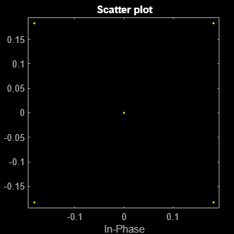
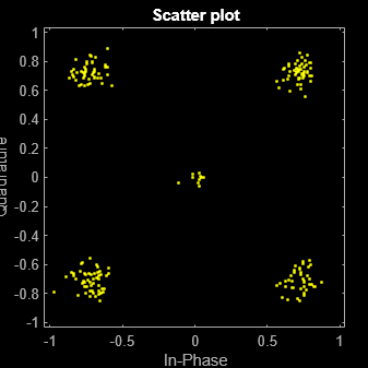
txSig = txfilter(modData);

송신된 신호의 성상도 다이어그램은 scatterplot 항목을 사용하여 표시할 수 있습니다. 신호가 필터 출력에서 오버샘플링되므로 산점도 플롯에 성상도 점 간의 천이 경로가 표시되지 않도록 심볼당 샘플 수만큼 데시메이션해야 합니다. 신호에 타이밍 오프셋이 있는 경우 해당 타이밍 오프셋을 입력 파라미터로 제공하여 타이밍 오프셋이 보정된 신호 성상도를 표시할 수 있습니다.

scatterplot(txSig,sps)

Figure Scatter Plot contains an axes object. The axes object with title Scatter plot, xlabel In-Phase, ylabel Quadrature contains a line object which displays its values using only markers. This object represents Channel 1.

또는 심볼당 샘플 수와 필요한 경우 타이밍 오프셋을 지정하여 comm.ConstellationDiagram 항목을 사용할 수 있습니다. 또한 comm.ConstellationDiagram을 사용하여 기준 성상도를 표시할 수 있습니다.

성상도 다이어그램을 만들고 SamplesPerSymbol 속성을 신호의 오버샘플링 인자로 설정합니다. 성상도 다이어그램을 지정하여 마지막 100개 샘플만 표시합니다. 이렇게 하면 RRC 필터가 처음 FilterSpanInSymbols개 샘플 동안 출력하는 0 값을 숨길 수 있습니다.

constDiagram = comm.ConstellationDiagram( ...
    SamplesPerSymbol=sps, ...
    SymbolsToDisplaySource='Property', ...
    SymbolsToDisplay=100);

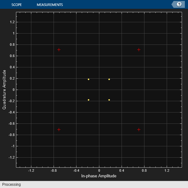
송신된 신호의 성상도 다이어그램을 표시합니다.

constDiagram(txSig)

신호를 기준 성상도와 일치시키려면 필터의 이득을 OutputSamplesPerSymbol 속성의 제곱근으로 설정하여 필터를 정규화합니다. 이 속성은 앞에서 sps로 지정되었습니다. 필터 이득은 조정이 불가능하므로 이 값을 변경하기 전에 객체를 해제해야 합니다.

release(txfilter)
txfilter.Gain = sqrt(sps);

변조 신호를 정규화된 필터에 통과시킵니다.

txSig = txfilter(modData);

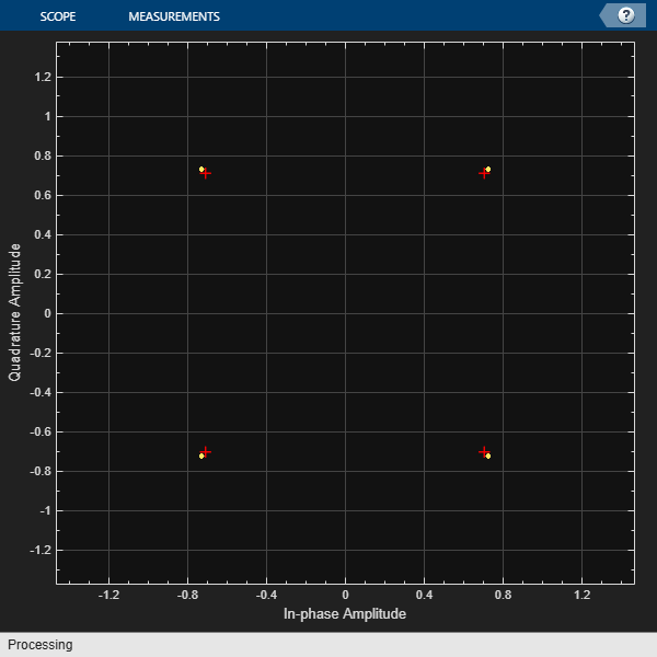
정규화된 신호의 성상도 다이어그램을 표시합니다. 데이터 점과 기준 성상도가 거의 중첩됩니다.

constDiagram(txSig)

송신된 신호를 더 명확하게 보려면 ShowReferenceConstellation 속성을 false로 설정하여 기준 성상도를 숨깁니다.

constDiagram.ShowReferenceConstellation = false;

txSig를 AWGN 채널에 통과시켜 잡음 있는 신호를 생성합니다.

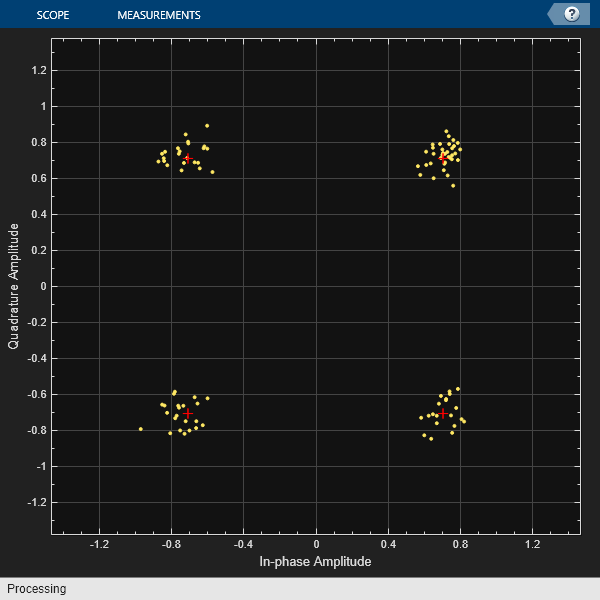
rxSig = awgn(txSig,20,'measured');

기준 성상도를 표시하고 수신된 신호 성상도를 플로팅합니다.

constDiagram.ShowReferenceConstellation = true;
constDiagram(rxSig)

scatterplot으로도 이 잡음 있는 신호를 볼 수 있지만, scatterplot을 사용하면 기준 성상도를 추가하는 내장 옵션이 제공되지 않습니다.

scatterplot(rxSig,sps)

참고 항목

Visualize RF Impairments | View Constellation of Modulator Block