timingEstimate

R2026b

Estimate timing offset for communication signals

Since R2024a

Syntax

[offset,normcorr] = timingEstimate(waveform,refsig)

[offset,normcorr] = timingEstimate(waveform,refsig,Name=Value)

Description

[offset,normcorr] = timingEstimate(waveform,refsig) performs timing estimation by cross-correlating the input waveform and a known reference signal. For more information, see Algorithms.

[offset,normcorr] = timingEstimate(waveform,refsig,Name=Value) specifies additional name-value arguments for detection threshold and window length.

Examples

Estimate Timing Offset of QPSK Signals

Generate a QPSK reference signal and input waveform. Fix the random seed.

 s = rng(123);
refSignal = pskmod(randi([0 3],[512 1]),4,pi/4);
waveform = pskmod(randi([0 3],[512 1]),4,pi/4);

Check the timing offset by using the reference signal as both inputs. Expected offset is 0.

offset1 = timingEstimate(refSignal,refSignal)

offset1 = 
0

Check the timing offset between the input waveform and the reference signal.

offset2 = timingEstimate(waveform,refSignal) % Expected offset is []

offset2 =

     []

offset3 = timingEstimate([zeros(5,1);refSignal],refSignal) % Expected offset is 5

offset3 = 
5

offset4 = timingEstimate([refSignal(2:end);0],refSignal) % Expected offset is -1

offset4 = 
-1

Generate a noise waveform input to compare with the reference signal.

noisyWaveform = awgn(refSignal,-15,'measured');

Estimate the timing offset and the normalized correlation magnitude between the noisy waveform and the reference signal.

[offset5, normCorr] = timingEstimate(noisyWaveform,refSignal) % Expected offset is []

offset5 =

     []

normCorr = 1023×1

    0.0442
    0.0198
    0.0066
    0.0462
    0.0556
    0.0391
    0.0425
    0.0149
    0.0185
    0.0532
    0.0680
    0.0080
    0.0284
    0.0642
    0.0193
      ⋮

Adjust the threshold to control the probability of missed detection. If needed, collect more normalized correlation data.

histogram(normCorr(:)) 

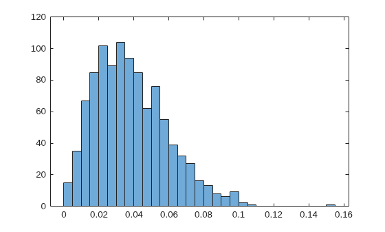
offset6 = timingEstimate(noisyWaveform,refSignal,Threshold=0.05) % Expected offset is 0

offset6 = 
0

Restore random seed.

rng(s);

Use WindowLength to Reduce Intersymbol Interference

Adjust the window length for a timing offset estimate to reduce intersymbol interference (ISI) in orthogonal frequency division multiplexing (OFDM) transmission.

Specify the OFDM parameters.

nfft = 512;
cplen = 16;
symLen = nfft + cplen;
nullIdx = [1:6 nfft/2+1 nfft-5:nfft]';
numDataCarrs = nfft-length(nullIdx);
modOrder = 64;
 

Generate the OFDM signal. Fix the random seed.

s = rng(123);
numSym = 100;
srcBits = randi([0,1], [numDataCarrs*log2(modOrder) numSym+2]);
ofdmData = qammod(srcBits,modOrder,InputType='bit', ...
            UnitAveragePower=true);
txSignal = ofdmmod(ofdmData,nfft,cplen,nullIdx); 

Use the second OFDM symbol as a reference signal.

refSig = txSignal(symLen+(1:symLen));

Generate a channel filter randomly. Make h(4) the biggest peak.

h = 10*randn(cplen+1,1,'like',1j);
h(4) = h(4)/abs(h(4))*(2*max(abs(h))); 

Pass reference signal through a filter. Add delay and noise.

rxSignal = awgn([zeros(213,1);filter(h,1,txSignal)], ...
           70,"measured");
 

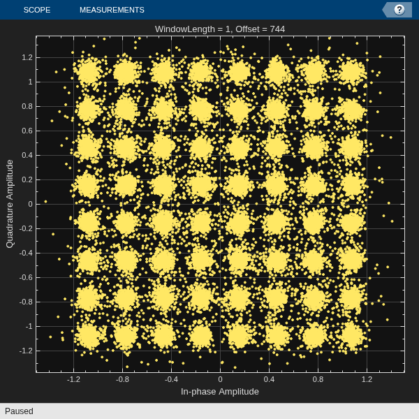
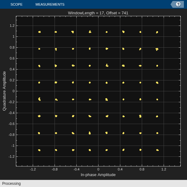
With the WindowLength property equal to the default value, the estimated timing offset points to the largest peak in the channel impulse response. But just using the default value for window length may not provide the timing offset required for reducing ISI. With the WindowLength=cplen+1, the function focuses on a window that is the length of the cyclic prefix (cplen) plus one sample. Then estimated timing offset shifts as much energy of the channel impulse response as possible into the cyclic prefix region of an OFDM symbol, aligning the timing offset with the received signal and reducing the ISI.

windowLenVec = [1 (cplen+1)];
 for k = 1:length(windowLenVec)
    % Get timing estimate
    offset = timingEstimate(rxSignal,refSig,WindowLength=windowLenVec(k));
    % Demodulate signal
    rxofdmData = ofdmdemod(rxSignal(offset+(1:symLen*numSym)), ...
                 nfft,cplen,cplen,nullIdx).';
    % Find the best possible equalizer by using
    % known data
    equalizerCoef = zeros(numDataCarrs,1);
     for n = 1:numDataCarrs
         equalizerCoef(n) = rxofdmData(:,n)\(ofdmData(n,1+(1:numSym)).');
     end
    % Equalize signal
    eqData = rxofdmData*diag(equalizerCoef);
    % Plot constellation diagram for all subcarriers
    % Set WindowLength=cplen+1 leads to a timing estimate that reduces ISI
    constdiag{k} = comm.ConstellationDiagram(ShowReferenceConstellation=false);
    constdiag{k}.Title = ['WindowLength = ' num2str(windowLenVec(k))...
                          ', Offset = ' num2str(offset)];
    constdiag{k}(eqData(:));
  end

Restore the random seed.

  rng(s); 

Input Arguments

waveform — Input waveform

T-by-N_Rx matrix

Input waveform, specified as a T-by-N_Rx matrix where:

• T is the number of time domain samples in the input signal.

• N_Rx is the number of receive antennas.

Data Types: double | single

refsig — Reference signal

L-by-N_Tx matrix

Reference signal, specified as an L-by-N_Tx matrix where:

• L is the number of time domain samples in the reference signal.

• N_Tx is the number of transmit streams.

Data Types: double | single

Name-Value Arguments

Specify optional pairs of arguments as Name1=Value1,...,NameN=ValueN, where Name is the argument name and Value is the corresponding value. Name-value arguments must appear after other arguments, but the order of the pairs does not matter.

Example: Z = timingEstimate(Y,M,Threshold=0.25);

Threshold — Detection threshold

0.2 (default) | real scalar in the range [0, 1]

Detection threshold, specified as a real scalar in the range [0, 1]. For any normalized cross-correlation magnitude greater than or equal to the threshold value, the function concludes that the waveform includes a reference signal. For more information on threshold value, see Tips.

Data Types: single | double

WindowLength — Window length of consecutive samples

1 (default) | positive integer | ...

Window length of consecutive samples, specified as a positive integer.

Data Types: single | double

Output Arguments

offset — Estimated timing offset

scalar integer | empty array

Estimated timing offset, returned as an integer, given by an integer number of samples relative to the first sample of the input waveform.

• If the offset is nonnegative, waveform(offset + (1:L),:) is a good match to the reference signal.

• If offset is negative, the received waveform is late. waveform(1:(L + offset),:) is a good match to refsig(1-offset:L,:).

• If waveform is not a good match to refsig, the returned offset is an empty array.

normcorr — Normalized correlation magnitude

(T+L-1)-by-N_Rx-by-N_Tx array

Normalized correlation magnitude, returned as a (T+L-1)-by-N_Rx-by-N_Tx array. Each element in the array is a real value in the range [0, 1]. A larger value indicates a stronger correlation between the input waveform and the reference signal for the corresponding offset, receive antenna, and the transmit stream.

• If all values in normcorr are less than the default threshold of 0.2, the function returns an empty array for offset.

• If normcorr meets or exceeds the default threshold value, the function calculates offset from the NTx×NRx estimated channel impulse responses between the transmit streams and the receive antennas.

Tips

• The function perceives any nonreference signal portion of the received waveform as noise. To return an accurate timing estimate, adjusting the detection threshold may be necessary, but is a tradeoff between missed detections and increased false detections.

  • Increasing the threshold can result in missed detections.

  • Decreasing the threshold can lead to false detections.

  For more information, see Algorithms.

Algorithms

The timingEstimate function helps to calculate the timing offset by estimating the location of a reference signal in the received signal. This function has two key algorithm stages. Both algorithm stages use cross-correlation between the reference signal and the received waveform. The first stage confirms detection of the reference signal in the received waveform. If the reference signal is in the received waveform, then the second stage estimates the timing offset.

Stage 1: Detection Stage

The detection algorithm uses the principle of a matched filter or cross-correlator to detect the presence and location of a reference signal within a received waveform. In cross-correlation, you slide a reference or given signal across a received signal and calculate the similarity between the signal. A plot of the cross-correlation shows peaks in the cross-correlated signal indicate potential locations of the reference signal within the received signal at a particular time. Higher peaks indicate more the similarity between the reference signal and the received signal. The magnitude of the cross-correlation peaks are influenced by several factors, such as the energy of the reference signal, the energy of the received signal, and the noise level. You can normalize or scale the peaks for a more accurate detection of the given signal. Without appropriate scaling, it becomes harder to compare the correlation peaks, which makes the detection more difficult or inaccurate.

Consider this:

refSignal = 2.3*randn(256,1,'like',1j); % No need to have unit power

% Create the waveform by concatenating zeros, scaled reference signals, and more zeros.
waveform = [zeros(12,1);2*refSignal;zeros(45,1);0.2*refSignal];

% Add complex Gaussian noise to the waveform
waveform = waveform + 0.01*randn(size(waveform),'like',1j);

% Perform correlation by filtering the waveform with a flipped and conjugated reference signal.
corrResult = filter(conj(flipud(refSignal)),1,[waveform;zeros(length(refSignal)-1,1)]);
% Equivalent to xcorr(waveform,refSignal), without padded zeros.

% Plot the absolute value of the correlation result
figure(1)
plot(abs(corrResult))

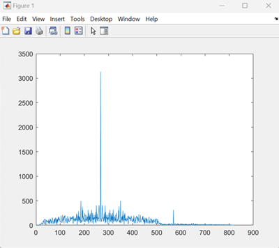
The peak in the graph corresponding to 0.2*refSignal is small compared to the peak corresponding to 2*refSignal. The difference is in the scaling values: 0.2 and 2. You also need to calculate the correlation result appropriately if there are no known scaling values.

To remove the effects of scaling factors 0.2 and 2, you can use the fact that for any column vectors u and v, abs(u'*v)/sqrt((u'*u)*(v'*v)) is always in the range [0, 1]. In this scenario, u is refSignal and v is a moving slice of waveform. Compute and store the magnitude squared of the waveform using a sliding window. Normalize the correlation magnitude to get two peaks very close to 1.

% Calculate the magnitude squared of the waveform using a sliding window.
waveformMagSq = filter(ones(size(refSignal)), 1, ...
    [real(waveform.*conj(waveform)); zeros(length(refSignal)-1, 1)]);

% Calculate the power of the reference signal.
refSigPower = real(refSignal'*refSignal);

% Normalize the correlation magnitude.
normCorrMag = abs(corrResult) ./ sqrt(waveformMagSq * refSigPower);

% Create a new figure for plotting
figure(2)

% Plot the normalized correlation magnitude.
plot(normCorrMag)

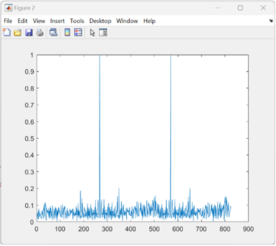
The function normalizes the correlation magnitude for each waveform from each receive antenna (1:N_Rx) and each reference signal from each transmit layer (1:N_Tx).

If one such normalization vector has a value that is equal to or greater than the detection threshold, then the function decides that the reference signal is present in the received waveform. To understand more about detection threshold, see Estimate Timing Offset of QPSK Signals.

Stage 2: Estimating Timing Offset

After confirming the presence of the reference signal in the received waveform, you need to estimate the timing offset You can use the autocorrelation properties of the reference signal to estimate the timing offset. Consider this example:

Generate a complex Gaussian noise reference signal with a specified scale factor. The scale factor of 3.4 is arbitrary and does not need to represent unit power.

refSignal = 3.4*randn(256,1,'like',1j);

Calculate the total energy of the reference signal by taking the conjugate transpose of the signal.

refTotalEnergy = real(refSignal'*refSignal);

Simulate the effect of the channel on the reference signal by filtering it with a given channel impulse response. The filter coefficients [0.8 0.5+0.2j -0.3+0.4j] represent the channel.

waveform = filter([0.8 0.5+0.2j -0.3+0.4j], 1, refSignal);

Add complex Gaussian noise to the waveform to simulate a noisy channel. The noise has a standard deviation of 0.01, scaled by the waveform's size.

waveform = waveform + 0.01*randn(size(waveform), 'like', 1j);

Perform cross-correlation between the received waveform and the reference signal. For this, filter the received waveform with the time-reversed and conjugated reference signal. The result is equivalent to the cross-correlation function without padding zeros at the end.

corrResult = filter(conj(flipud(refSignal)), 1, [waveform;zeros(length(refSignal)-1, 1)]);

Estimate the channel impulse response by normalizing the cross-correlation result with the total energy of the reference signal.

estImpulseResponse = corrResult / refTotalEnergy;

Extract the estimated channel impulse response starting from the sample immediately after the reference signal length. This portion of the impulse response should be close to the actual channel filter coefficients. Add the length of the reference signal to the index to account for the delay introduced by the filtering process.

estImpulseResponse(length(refSignal)+(0:2))

The result is expected to be close to [0.8; 0.5+0.2j; -0.3+0.4j].

In the above example, the computation assumes that the reference signal is present in the received waveform, and that the reference signal has good autocorrelation properties or the autocorrelation function is close to an impulse.

The timingEstimate function calculates estimated impulse response for each received waveform (1:N_Rx) and for the reference signal from each transmit layer (1:N_Tx). The function then sums the magnitude squared of the estimated impulse response over all N_Rx×N_Tx combinations.

The function uses this vector of total power to find which W consecutive samples in this vector have the largest sum. Here, W is the width of the window used to sum the power of estimated impulse response components. Subtracting the length of the reference signal from the one-based index of the first sample in these W consecutive samples gives the timing estimate. (If more than one set of W consecutive samples achieves the largest sum, then the smallest timing estimate is used.)

• If W = 1, the algorithm looks for a single peak in the total power vector.

• If W > 1, the algorithm considers a peak energy that spreads over multiple samples instead of one sample. You can set W to CPLEN + 1, where CPLEN is the cyclic prefix length of an OFDM symbol. This region is the potential start of the OFDM symbol. This algorithm is a heuristic to reduce intersymbol interference.

This algorithm provides a practical means to estimate the timing offset in a communication system by leveraging the autocorrelation properties of a reference signal and the received waveform's cross-correlation with it.

Extended Capabilities

GPU Arrays

Accelerate code by running on a graphics processing unit (GPU) using Parallel Computing Toolbox™.

For GPU processing, both waveform and refsig inputs must be a gpuArray object.

For more information, see Accelerate Simulation Using GPUs.

Version History

Introduced in R2024a

R2026a: Add GPU array support

The timingEstimate function adds support for gpuArray (Parallel Computing Toolbox) object processing to run code on a graphics processing unit (GPU).