Visualize Ambisonic Sound Field

This example shows how to visualize the directional information in an ambisonic signal.

Introduction

Ambisonics is a surround sound format that captures and reproduces sound in a 360-degree sphere. Rather than corresponding to specific loudspeakers, the audio channels of an ambisonic signal contain a loudspeaker-independent representation of the sound field. Therefore, it is not straightforward to visualize the characteristics of the sound field by directly inspecting the individual ambisonic channels.

In this example, you visualize the sound field by first decoding the ambisonic signal to a virtual loudspeaker setup. You then measure the power at each virtual loudspeaker and use these measurements to visualize the directional information of the signal.

Create Ambisonic Signal

Start by creating a simple ambisonic signal that encodes two distinct sound sources.

Define the ambisonic order.

order = 3;

Define the azimuth and elevation (in degrees) of the two sound sources.

source1 = [-90 -45];
source2 = [90 45];
sources = [source1; source2];

Create the ambisonic encoding matrix.

E = ambisonicEncoderMatrix(order,sources);

Create the ambisonic signal by encoding 2 channels of audio corresponding to the 2 sources.

frameSize = 512;
audioIn = randn(frameSize,2);
X = audioIn*E;

The ambisonic signal is an N-by-L matrix, where N is the audio signal length, and L = (order+1)^2.

size(X)

ans = 1×2

   512    16

Create Virtual Loudspeaker Setup

Create a t-design loudspeaker setup. T-designs ensure that the loudspeakers are evenly distributed over the surface of a sphere, providing uniform coverage and accurate spatial audio reproduction.

Get the cartesian coordinates (in degrees) of the loudspeakers.

loudspeakerXYZ = getTDesign();

Plot the loudspeaker locations in space.

figure
k1 = convhull(loudspeakerXYZ(:,1),loudspeakerXYZ(:,2),loudspeakerXYZ(:,3),Simplify=true);
trisurf(k1,loudspeakerXYZ(:,1),loudspeakerXYZ(:,2),loudspeakerXYZ(:,3),FaceColor="cyan")
axis equal
xlabel("x (m)")
xlabel("y (m)")
xlabel("z (m)")

Convert the loudspeaker cartesian coordinates to spherical coordinates (in degrees):

loudspeakerSph = zeros(size(loudspeakerXYZ,1),2);
[loudspeakerSph(:,1),loudspeakerSph(:,2)] = cart2sph(loudspeakerXYZ(:,1),loudspeakerXYZ(:,2),loudspeakerXYZ(:,3));
loudspeakerSph = 180*loudspeakerSph/pi;

Decode Ambisonic Signal

Create the ambisonic decoder matrix.

D = ambisonicDecoderMatrix(order,loudspeakerSph);

Decode the ambisonic signal onto the virtual loudspeaker setup.

Y = X*D;

The decoded signal is an N-by-M matrix, where N is the audio signal length, and M is the number of loudspeakers.

size(Y)

ans = 1×2

   512   240

Visualize Sound Field

Compute the power of the signals at each loudspeaker.

p = sum(Y.^2)./size(Y,1);

Create a mesh grid corresponding to the loudspeaker locations.

azi = loudspeakerSph(:,1);
ele = loudspeakerSph(:,2);

aziLin = linspace(min(azi), max(azi), 240);
eleLin = linspace(min(ele), max(ele), 240);
[AZ,EL] = meshgrid(aziLin, eleLin);

Interpolate the measured power values to the grid points.

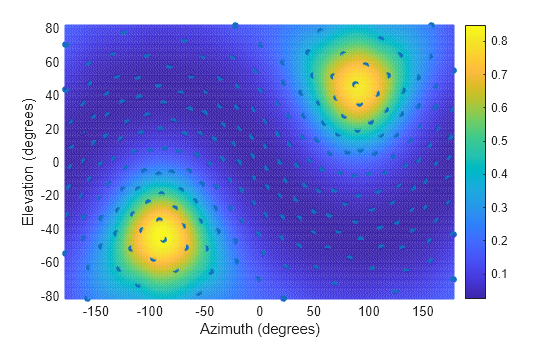
P = griddata(azi,ele,p,AZ,EL,'v4');

Visualize the sound field by plotting the interpolated mesh. Overlay the mesh with the power values from the individual speakers.

Notice the two areas of strong audio activity correspond to the locations of the two sound sources.

figure
mesh(AZ,EL,P)
axis tight
hold on
plot3(azi,ele,p,'.',MarkerSize=15)
view(2)
xlabel("Azimuth (degrees)")
ylabel("Elevation (degrees)")
colorbar

Visualize Sound Field in Real-Time

You can visualize the sound field in a streaming, real-time simulation.

Create an ambisonic encoder plugin class with two sound sources.

sources = [200 -45; 90 45];
audioexample.ambisonics.ambiGenerateEncoderPlugin("myAmbiEncoder", order, sources)

Instantiate an ambisonic encoder.

 enc = myAmbiEncoder;

Launch the parameter tuner of the encoder. You can modify the location of the two sound sources as the simulation is running.

parameterTuner(enc)

To avoid interpolating over the sense grid inside the simulation loop, use an extended virtual loudspeaker setup encompassing all points on the dense grid.

azi(azi<0) = azi(azi<0)+360;
aziLin = linspace(min(azi), max(azi), 240);
eleLin = linspace(min(ele), max(ele), 240);
[AZ,EL] = meshgrid(aziLin, eleLin);

D = ambisonicDecoderMatrix(order,[AZ(:) EL(:)]);

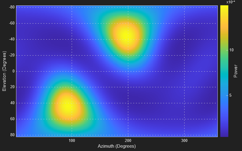
Use a matrix viewer scope to visualize the sound field.

m = dsp.MatrixViewer(XDataMode = "Custom",...
    YDataMode = "Custom",...
    CustomXData = aziLin,...
    CustomYData = eleLin,...
    XLabel = "Azimuth (Degrees)",...
    YLabel = "Elevation (Degrees)",...
    ColorBarLabel = "Power");

Create a moving average filter to smooth the power measurements at the speakers.

mavrg = dsp.MovingAverage(Method="Exponential weighting",ForgettingFactor=.1);

Execute the simulation loop to visualize the sound field in real-time. Tune the location of the sources and observe the changes in the displayed sound field.

show(m)
numIter = 100;
for index=1:numIter
     
    % Two-channel audio signal (2 sources)
    xin = rand(frameSize,2);

    % Create ambisonic signal
    XAmbi = process(enc,xin);

    % Decode the ambisonic signal
    YAmbi = XAmbi*D;

    % Compute power at each loudspeaker
    p = sum(YAmbi.^2)/frameSize;

    % Smooth the power measurements
    p = mavrg(p);

    P = reshape(p,size(AZ,1),size(AZ,2));

    % Visualize sound field
    m(P)

    drawnow limitrate
end