Model and Analyze a Microspeaker

R2026b

Since R2026b

This example shows how to model a microspeaker mounted on an infinite baffle using the Simscape™ Acoustics library. Microspeakers are miniature transducers commonly found in headphones, earbuds, and portable devices. Although they share the same electrodynamic operating principle as traditional loudspeakers, their compact geometry introduces additional acoustic elements, such as front and rear cavities, cover holes, and rear vents, that significantly influence the frequency response.

This example proceeds in two stages:

1. First, build the microspeaker from individual electrical, mechanical, and acoustic elements (resistances, compliances, inertances) to illustrate the underlying physics.

2. Then, replace the low-level network with the Microspeaker block from the Acoustics library, which encapsulates the same functionality in a single, parameterizable component.

After establishing the baseline frequency response, the example performs a parametric study to show how key geometric parameters affect the sound pressure level (SPL).

Open the Low-Level Model

The model Microspeaker represents the microspeaker using discrete lumped-parameter elements. The electrical domain captures the voice coil resistance and inductance. The mechanical domain represents the diaphragm mass, suspension compliance, and damping. The acoustic domain models the front and rear cavities as compliances, the cover holes as series inertance-resistance pairs, and the rear vents similarly.

model = "Microspeaker";
open_system(model);

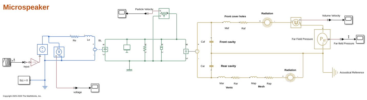
Run a short time-domain simulation to verify the model.

sim(model,.2);
bdclose(model)

Linearize the Library Block Model

The model MicrospeakerBlock.slx uses the composite Microspeaker block from the Acoustics library. This block encapsulates the full electro-mechano-acoustic network in a single component with parameterized geometry, making it convenient for design exploration.

model = "MicrospeakerBlock";
open_system(model);

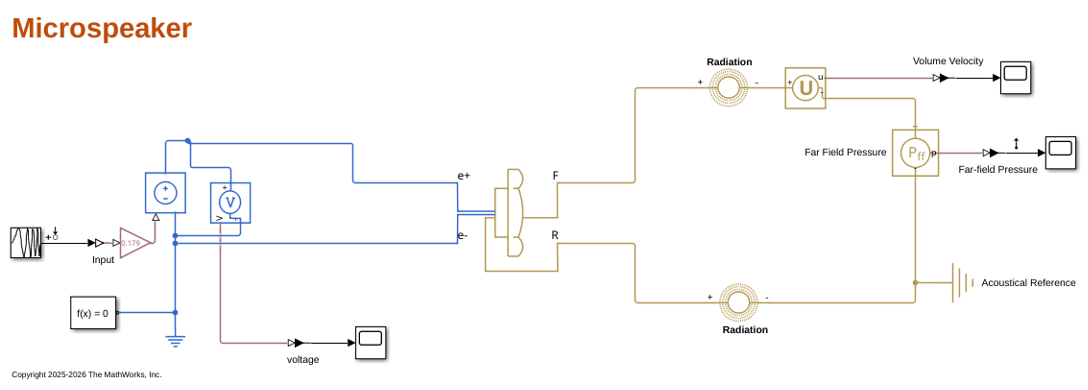
To characterize the microspeaker, perform frequency-domain analysis by linearizing the model. This is equivalent to extracting the time-domain output and computing the Fourier transform, but is more computationally efficient.

Define the linearization input and output points.

io(1) = linio("MicrospeakerBlock/Chirp Signal",1, "input");              % input perturbation
io(2) = linio("MicrospeakerBlock/Far-field Pressure",1, "output");       % output measurement

Linearize the model and extract the Bode magnitude response.

linsys = linearize(model,io);       % linearize model
[mag, ~, wout] = bode(linsys);      % extract results

Convert the angular frequency to Hz and compute the sound pressure level in dB SPL. The SPL is defined as:

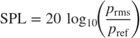
where the reference pressure in air is .

p_ref = 20e-6;                    % reference pressure in air (Pa)
freq = wout./(2*pi);              % convert rad/s to Hz
SPL = 20.*log10(mag(:)./p_ref);   % calculate dB SPL

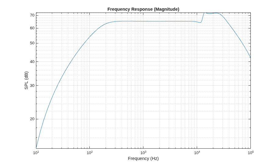
Plot the baseline frequency response.

figure(1)
loglog(freq, SPL);
xlim([10 100e3]);
title("Frequency Response (Magnitude)");
xlabel("Frequency (Hz)");
ylabel("SPL (dB)");
grid on
hold on

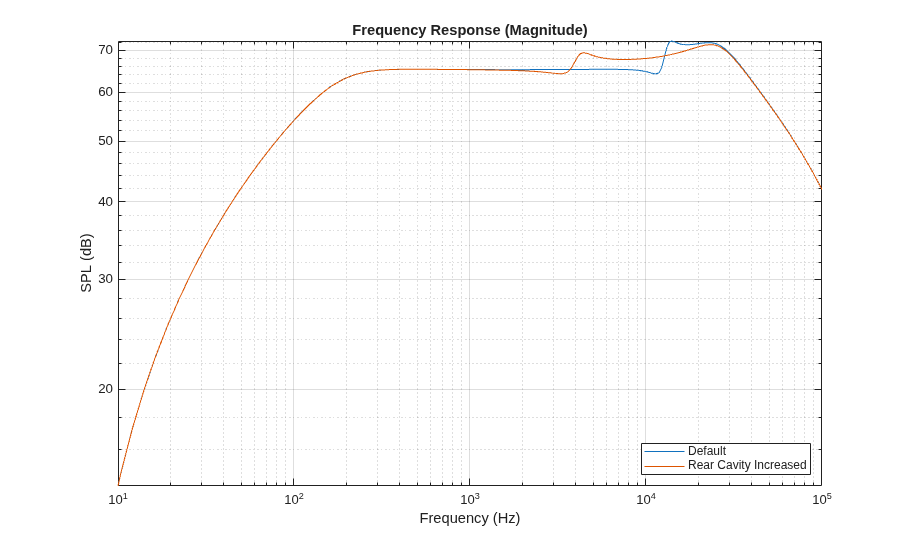
Increase Rear Cavity Volume

The rear cavity acts as an acoustic compliance behind the diaphragm. Increasing its volume by a factor of 10 reduces the acoustic stiffness, which lowers the fundamental resonance frequency and increases the low-frequency SPL. Physically, a larger rear cavity gives the diaphragm more room to move, improving bass response at the cost of a downward shift in the resonance peak.

blockName = model + "/Microspeaker";
set_param(blockName,"Vb", "1.01646e-6");

Linearize the modified model.

linsys = linearize(model,io);           % linearize model
[mag, ~, wout] = bode(linsys);          % extract results
freq = wout./(2*pi);                    % convert rad/s to Hz
SPL = 20.*log10(mag(:)./p_ref);         % calculate dB SPL

Plot the results.

loglog(freq, SPL);
xlim([10 100e3]);
title("Frequency Response (Magnitude)");
xlabel("Frequency (Hz)");
ylabel("SPL (dB)");
legend("Default", "Rear Cavity Increased", "Location", "southeast");

Restore the default value.

set_param(blockName,"Vb", "1.01646e-7");

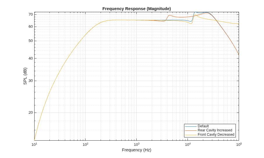
Decrease Front Cavity Volume

The front cavity is the air volume between the diaphragm and the front cover. In the lumped-parameter model, it behaves as an acoustic compliance. Decreasing its volume by a factor of 10 stiffens the front acoustic path, shifting the associated resonance to higher frequencies. This can create a pronounced high-frequency peak or reduce the mid-range output, depending on the coupling with other elements.

set_param(blockName,"Vf", "1.02453e-8");

Linearize the modified model.

linsys = linearize(model,io);       % linearize model
[mag, ~, wout] = bode(linsys);      % extract results
freq = wout./(2*pi);                % convert rad/s to Hz
SPL = 20.*log10(mag(:)./p_ref);     % calculate dB SPL

Plot the results.

loglog(freq, SPL);
xlim([10 100e3]);
title("Frequency Response (Magnitude)");
xlabel("Frequency (Hz)");
ylabel("SPL (dB)");
legend("Default", "Rear Cavity Increased", "Front Cavity Decreased", "Location", "southeast");
grid on
hold on

Restore the default value.

set_param(blockName,"Vf", "1.02453e-7");

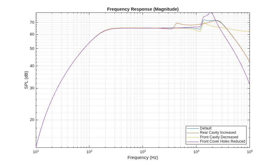
Reduce Front Cover Holes

The holes on the front cover act as short acoustic tubes connecting the front cavity to the outside air. Each hole contributes an acoustic inertance (mass) and resistance in series. For identical holes in parallel, the effective inertance and resistance are reduced by a factor of . Here the number of holes is halved (36 to 18), the hole radius is halved, and the cover thickness is halved. The net effect is a significant increase in the front acoustic impedance: the air must squeeze through fewer, smaller openings, which attenuates high-frequency radiation and introduces additional damping. The result is a roll-off or suppression of the high-frequency SPL peaks.

set_param(blockName,"thikf", "0.00015");
set_param(blockName,"rf", "0.00025");
set_param(blockName,"Nf", "18");

Linearize the modified model.

linsys = linearize(model,io);           % linearize model
[mag, ~, wout] = bode(linsys);          % extract results
freq = wout./(2*pi);                    % convert rad/s to Hz
SPL = 20.*log10(mag(:)./p_ref);         % calculate dB SPL

Plot the results.

loglog(freq, SPL);
xlim([10 100e3]);
title("Frequency Response (Magnitude)");
xlabel("Frequency (Hz)");
ylabel("SPL (dB)");
legend("Default", "Rear Cavity Increased", "Front Cavity Decreased", "Front Cover Holes Reduced", ...
    "Location", "southeast");

Restore the default values.

set_param(blockName,"thikf", "0.0003");
set_param(blockName,"rf", "0.0005");
set_param(blockName,"Nf", "36");

Increase Rear Vent

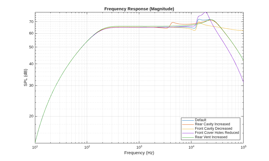
The rear vents are small holes in the back plate that allow controlled acoustic leakage from the rear cavity to the ambient. They form a low-pass acoustic filter: at low frequencies, sound leaks through the vents and partially cancels the front radiation (acoustic short-circuit), reducing bass output. At higher frequencies, the acoustic inertance of the vent air blocks the leakage and the rear cavity acts as sealed.

Increasing the vent area (doubling the number of holes from 8 to 16, doubling the radius, and reducing the thickness) lowers both the resistance and inertance of the rear path. This extends the acoustic short-circuit to higher frequencies, steepening the low-frequency roll-off and effectively raising the system's high-pass corner frequency.

set_param(blockName,"thikv", "0.001");
set_param(blockName,"rv", "0.00082");
set_param(blockName,"Nv", "16");

Linearize the modified model.

linsys = linearize(model,io);       % linearize model
[mag, ~, wout] = bode(linsys);      % extract results
freq = wout./(2*pi);                % convert rad/s to Hz
SPL = 20.*log10(mag(:)./p_ref);     % calculate dB SPL

Plot the results.

loglog(freq, SPL);
xlim([10 100e3]);
title("Frequency Response (Magnitude)");
xlabel("Frequency (Hz)");
ylabel("SPL (dB)");
legend("Default", "Rear Cavity Increased", "Front Cavity Decreased", ...
    "Front Cover Holes Reduced", "Rear Vent Increased", ...
    "Location", "southeast");

Restore the default values.

set_param(blockName,"thikv", "0.005");
set_param(blockName,"rv", "0.00041");
set_param(blockName,"Nv", "8");

Close the model.

bdclose(model)

References

• Shiah, Y. C., Her, H.-C., & Huang, J. H. (2008). Parametric analysis for a miniature loudspeaker used in cellular phones. Journal of Applied Physics, 104, 10.1063/1.3021098.

• Huang, J. H., Her, H.-C., Shiah, Y. C., & Shin, S.-J. (2008). Electroacoustic simulation and experiment on a miniature loudspeaker for cellular phones. Journal of Applied Physics, 103, 10.1063/1.2837112.

Copyright 2025-2026 The MathWorks, Inc.