Equiangular Spiral Antenna Design Investigation
This example compares results published in [1] for a two-arm equiangular spiral antenna on foamclad backing( 1), with those obtained using the toolbox model of the spiral antenna of the same dimensions. The spiral antennas belong to the class of frequency-independent antennas. In theory, such antennas may possess an infinite bandwidth when made infinitely large. In reality, a finite feeding region has to be established and the outer extent of the spiral antenna has to be truncated.
Equiangular Spiral Antenna Parameters
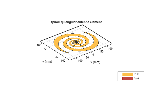
The equiangular spiral antenna is defined by a radius that grows exponentially with the winding angle. The expansion of the spiral is controlled by a factor called the growth rate. In [1], the authors use the angle between the tangent and radial vectors at any point on the spiral to define the growth rate. The inner radius of the spiral is the radius of the feeding structure, while the outer radius is the furthest extent on either arm of the spiral. Note, that the spiral arms are truncated to minimize reflections arising from the ends.
psi = 79*pi/180;
a = 1/tan(psi);
Ri = 3e-3;
Ro = 114e-3;
Create the Antenna
The parameters defined earlier are used to create an equiangular spiral antenna.
sp = spiralEquiangular(GrowthRate=a,InnerRadius=Ri,OuterRadius=Ro);
SpiralFig = figure;
show(sp)
Impedance Behavior of the Equiangular Spiral
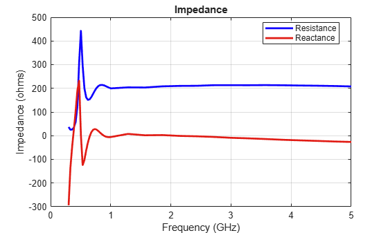
The impedance behavior of the spiral antenna shows multiple resonances at the low frequency band, before achieving a relatively constant resistance and reactance with increasing frequency. To capture these resonances, split up the frequency band into two parts. Sample the lower frequency band with a finer spacing and higher frequency band with courser spacing.
Nf1 = 25;
Nf2 = 15;
fband1 = linspace(0.3e9,1e9,Nf1);
fband2 = linspace(1e9,5e9,Nf2);
freq = unique([fband1,fband2]);
SpiralImpFig = figure;
impedance(sp,freq);
Boresight Directivity Variation with Frequency
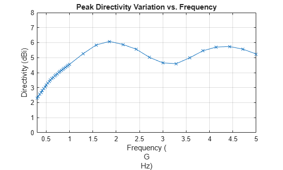
Spiral antennas by themselves are bidirectional radiators. To suppress unwanted radiation, they are used with a ground plane and dielectric backing. The toolbox model of the equiangular spiral does not have a ground plane or the backing material.
SpiralDVarFig = figure;
D = zeros(1,length(freq));
for p = 1:length(freq)
    D(p) = pattern(sp,freq(p),0,90);
end
f_eng = freq./1e9;
f_str = 'G';
plot(f_eng,D,'x-')
grid on
axis([f_eng(1) f_eng(end) 0 8 ])
xlabel(["Frequency (" f_str "Hz)"])
ylabel("Directivity (dBi)")
title("Peak Directivity Variation vs. Frequency")
Discussion on Results
Paper [1], compares two types of backing - Foamclad, and Rogers substrate. Since Foamclad, has relative permittivity nearly equivalent to free space, we use this for comparing results with the metal-only spiral from the toolbox. The Foamclad-backed spiral in [1] achieves a nearly constant resistance of 188 after 1 GHz and the reactance varies between approximately 10 - 20 . This result agrees very well with the equiangular spiral model from the toolbox. The boresight directivity for the toolbox model of the equiangular spiral varies between 4.5 - 6 dB between 1-5 GHz. This also matches well with the results from [1].
Reference
[1] M. McFadden, W. R. Scott, "Analysis of the Equiangular Spiral Antenna on a Dielectric Substrate," IEEE Transactions on Antennas and Propagation, vol.55, no.11, pp.3163-3171, Nov. 2007.