showConvergenceTrend

Plot optimization convergence trend

Since R2025a

Syntax

showConvergenceTrend(obj)

Description

showConvergenceTrend(obj) plots the optimization convergence trend.

Examples

Optimize Dipole Antenna for Directivity

Create a dipole antenna resonating at 75 MHz and calculate its maximum directivity.

Choose its length and width as design variables. Provide lower and upper bounds of length and width.

referenceAnt = design(dipole,75e6);
InitialDirectivity = max(max(pattern(referenceAnt,75e6)))

InitialDirectivity = 
2.1002

length_lb = 3; % Lower bound for length
length_ub = 7; % Upper bound for length
width_lb = 0.11; % Lower bound for width
width_ub = 0.13; % Upper bound for width
Bounds = [length_lb width_lb; length_ub width_ub];

Use the SADEA optimizer to optimize this dipole antenna for its directivity. Specify an evaluation function for optimization using the CustomEvaluationFunction property of the OptimizerSADEA object. The evaluation function used in this example is defined at the end of this example.

s = OptimizerSADEA(Bounds);
s.CustomEvaluationFunction = @customEvaluationOnlyObjective;

Validate the optimizer setup.

validateSetup(s)

ans = logical
   1

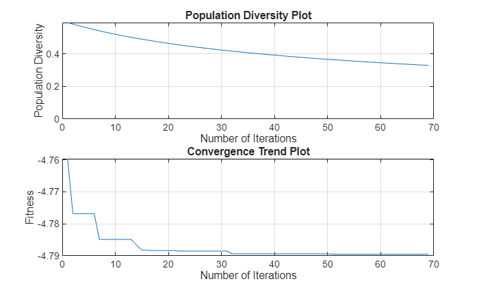
Run the optimization for 100 iterations.

figure
optimizeWithPlots(s,100);

View the best member data.

bestDesign = s.getBestMemberData

bestDesign = 
  bestMemberData with properties:

             member: [4.8004 0.1100]
       performances: -4.7895
            fitness: -4.7895
    bestIterationId: 72

bestDesignValues = bestDesign.member

bestDesignValues = 1×2

    4.8004    0.1100

Update the reference antenna with best design values from the optimizer. Calculate directivity of the optimized design.

Observe an increase in directivity value after optimization.

referenceAnt.Length = bestDesignValues(1);
referenceAnt.Width = bestDesignValues(2);
postOptimizationDirectivity = max(max(pattern(referenceAnt,75e6)))

postOptimizationDirectivity = 
4.7895

View the surrogate model data used for prediction.

InitialData = s.getInitializationData

InitialData = 
  initializationData with properties:

         members: [30×2 double]
    performances: [30×1 double]
         fitness: [30×1 double]

View the data for all iterations.

iterData = s.getIterationData

iterData = 
  iterationData with properties:

         members: [75×2 double]
    performances: [75×1 double]
         fitness: [75×1 double]

Check if the algorithm has converged.

ConvergenceFlag = s.isConverged

ConvergenceFlag = logical
   1

Check how many times the evaluation function is computed.

numEvaluations = s.getNumberOfEvaluations

numEvaluations = 
105

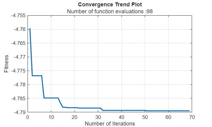
Plot the convergence trend.

s.showConvergenceTrend

This code defines the evaluation function used in this example.

function fitness = customEvaluationOnlyObjective(designVariables)
    
        % Create geometry
        ant = design(dipole,75e6);
        ant.Length = designVariables(1);
        ant.Width = designVariables(2);
    
        % Calculate directivity
        % Optimizer always minimizes the objective hence reverse the sign to maximize gain.
        objective = max(max(pattern(ant,75e6)));
        objective = -objective; 
        
        % As there are no constraints, fitness equals objective.
        fitness = objective;
    
end

Input Arguments

obj — Optimizer

OptimizerSADEA object | OptimizerTRSADEA object

Optimizer, specified as an OptimizerSADEA or OptimizerTRSADEA object. The function plots the convergence trend associated with the optimizer object specified in obj.

Example: OptimizerSADEA

Version History

Introduced in R2025a