Model-Based Network Latency Analysis of Automotive System

R2026b

Since R2026a

This example shows how to perform a pathing analysis for latency in a car physical architecture using System Composer™ functions. A pathing analysis is a series of decision points to find the shortest, optimal path between nodes. A pathing analysis informs you of changes in the latency analysis when the path changes so that you understand the values associated with a certain path. A shortest path calculation can be different based on which architectures you run it on and which variants are active, allowing you to choose the best configuration and design choices that lead to the best outcome. For example, you can change the hardware to make the latency faster after doing a trade off analysis on the additional cost.

Network latency is the time delay experienced as data travels from source to destination, influenced by factors such as distance, congestion, and intermediary devices. Analyzing latency involves measuring and diagnosing these delays, enabling targeted optimizations to improve network performance. In this example, network latency between elements is encoded in a stereotyped property called Latency.

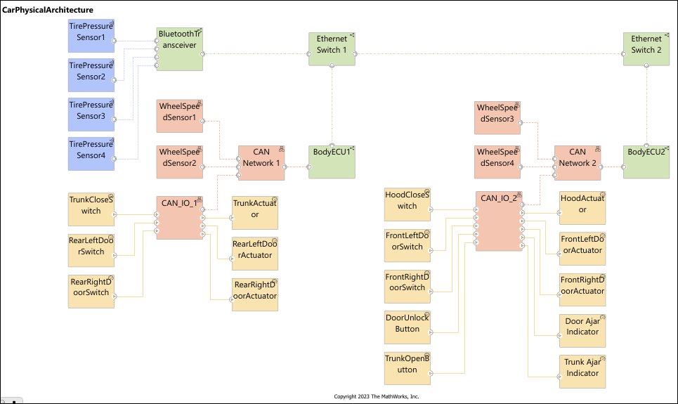
To visualize the shortest path network analysis for the car physical architecture model CarPhysicalArchitecture, you must first define a starting point and ending point. The starting point is the TrunkOpenButton component and the ending point is the TrunkActuator component, representing the time it takes from pressing a button to open the trunk and for the trunk to open.

Run the runAnalysis function.

runAnalysis

Total latency is 8

compPath = 28×1 cell
    {'LatencyAnalysis/TrunkOpenButton'       }
    {'LatencyAnalysis/TrunkOpenButton:DO0'   }
    {'LatencyAnalysis/CAN_IO_2:DI4'          }
    {'LatencyAnalysis/CAN_IO_2'              }
    {'LatencyAnalysis/CAN_IO_2:CAN'          }
    {'LatencyAnalysis/CAN Network 2:J3'      }
    {'LatencyAnalysis/CAN Network 2'         }
    {'LatencyAnalysis/CAN Network 2:J0'      }
    {'LatencyAnalysis/BodyECU2:CAN'          }
    {'LatencyAnalysis/BodyECU2'              }
    {'LatencyAnalysis/BodyECU2:Eth0'         }
    {'LatencyAnalysis/Ethernet Switch 2:Eth1'}
    {'LatencyAnalysis/Ethernet Switch 2'     }
    {'LatencyAnalysis/Ethernet Switch 2:Eth0'}
    {'LatencyAnalysis/Ethernet Switch 1:Eth1'}
    {'LatencyAnalysis/Ethernet Switch 1'     }
    {'LatencyAnalysis/Ethernet Switch 1:Eth2'}
    {'LatencyAnalysis/BodyECU1:Eth0'         }
    {'LatencyAnalysis/BodyECU1'              }
    {'LatencyAnalysis/BodyECU1:CAN'          }
    {'LatencyAnalysis/CAN Network 1:J0'      }
    {'LatencyAnalysis/CAN Network 1'         }
    {'LatencyAnalysis/CAN Network 1:J3'      }
    {'LatencyAnalysis/CAN_IO_1:CAN'          }
    {'LatencyAnalysis/CAN_IO_1'              }
    {'LatencyAnalysis/CAN_IO_1:DO0'          }
    {'LatencyAnalysis/TrunkActuator:DI0'     }
    {'LatencyAnalysis/TrunkActuator'         }

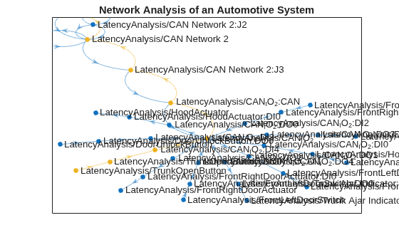
The total latency along the path is 8 ms. The network latency graph shows a visual representation of the result that shows a directed graph of the nodes in the shortest path between source and target zoomed in at the source, which is the start of the path at TrunkOpenButton. The shortest path in this pathing analysis is designated in yellow, while the full network is plotted in shades of blue. You can use this information to optimize your architecture with cost functions that minimize latency.