Nonlinear Logistic Regression
This example shows two ways of fitting a nonlinear logistic regression model. The first method uses maximum likelihood (ML) and the second method uses generalized least squares (GLS) via the function fitnlm from Statistics and Machine Learning Toolbox™.
Problem Description
Logistic regression is a special type of regression in which the goal is to model the probability of something as a function of other variables. Consider a set of predictor vectors where is the number of observations and is a column vector containing the values of the predictors for the th observation. The response variable for is where represents a Binomial random variable with parameters , the number of trials, and , the probability of success for trial . The normalized response variable is - the proportion of successes in trials for observation . Assume that responses are independent for . For each :
.
Consider modeling as a function of predictor variables .
In linear logistic regression, you can use the function fitglm to model as a function of as follows:
with representing a set of coefficients multiplying the predictors in . However, suppose you need a nonlinear function on the right-hand-side:
There are functions in Statistics and Machine Learning Toolbox™ for fitting nonlinear regression models, but not for fitting nonlinear logistic regression models. This example shows how you can use toolbox functions to fit those models.
Direct Maximum Likelihood (ML)
The ML approach maximizes the log likelihood of the observed data. The likelihood is easily computed using the Binomial probability (or density) function as computed by the binopdf function.
Generalized Least Squares (GLS)
You can estimate a nonlinear logistic regression model using the function fitnlm. This might seem surprising at first since fitnlm does not accommodate Binomial distribution or any link functions. However, fitnlm can use Generalized Least Squares (GLS) for model estimation if you specify the mean and variance of the response. If GLS converges, then it solves the same set of nonlinear equations for estimating as solved by ML. You can also use GLS for quasi-likelihood estimation of generalized linear models. In other words, we should get the same or equivalent solutions from GLS and ML. To implement GLS estimation, provide the nonlinear function to fit, and the variance function for the Binomial distribution.
Mean or model function
The model function describes how changes with . For fitnlm, the model function is:
Weight function
fitnlm accepts observation weights as a function handle using the 'Weights' name-value pair argument. When using this option, fitnlm assumes the following model:
where responses are assumed to be independent, and is a custom function handle that accepts and returns an observation weight. In other words, the weights are inversely proportional to the response variance. For the Binomial distribution used in the logistic regression model, create the weight function as follows:
fitnlm models the variance of the response as where is an extra parameter that is present in GLS estimation, but absent in the logistic regression model. However, this typically does not affect the estimation of , and it provides a "dispersion parameter" to check on the assumption that the values have a Binomial distribution.
An advantage of using fitnlm over direct ML is that you can perform hypothesis tests and compute confidence intervals on the model coefficients.
Generate Example Data
To illustrate the differences between ML and GLS fitting, generate some example data. Assume that is one dimensional and suppose the true function in the nonlinear logistic regression model is the Michaelis-Menten model parameterized by a vector :
myf = @(beta,x) beta(1)*x./(beta(2) + x);
Create a model function that specifies the relationship between and .
mymodelfun = @(beta,x) 1./(1 + exp(-myf(beta,x)));
Create a vector of one dimensional predictors and the true coefficient vector .
rng(300,'twister');
x    = linspace(-1,1,200)';
beta = [10;2];
Compute a vector of values for each predictor.
mu = mymodelfun(beta,x);
Generate responses from a Binomial distribution with success probabilities and number of trials .
n = 50;
z = binornd(n,mu);
Normalize the responses.
y = z./n;
ML Approach
The ML approach defines the negative log likelihood as a function of the vector, and then minimizes it with an optimization function such as fminsearch. Specify beta0 as the starting value for .
mynegloglik = @(beta) -sum(log(binopdf(z,n,mymodelfun(beta,x))));
beta0 = [3;3];
opts = optimset('fminsearch');
opts.MaxFunEvals = Inf;
opts.MaxIter = 10000;
betaHatML = fminsearch(mynegloglik,beta0,opts)
betaHatML = 2×1
9.9259
1.9720
The estimated coefficients in betaHatML are close to the true values of [10;2].
GLS Approach
The GLS approach creates a weight function for fitnlm previously described.
wfun = @(xx) n./(xx.*(1-xx));
Call fitnlm with custom mean and weight functions. Specify beta0 as the starting value for .
nlm = fitnlm(x,y,mymodelfun,beta0,'Weights',wfun)nlm =
Nonlinear regression model:
y ~ F(beta,x)
Estimated Coefficients:
Estimate SE tStat pValue
________ _______ ______ __________
b1 9.926 0.83135 11.94 4.193e-25
b2 1.972 0.16438 11.996 2.8182e-25
Number of observations: 200, Error degrees of freedom: 198
Root Mean Squared Error: 1.16
R-Squared: 0.995, Adjusted R-Squared 0.995
F-statistic vs. zero model: 1.88e+04, p-value = 2.04e-226
Get an estimate of from the fitted NonLinearModel object nlm.
betaHatGLS = nlm.Coefficients.Estimate
betaHatGLS = 2×1

    9.9260
    1.9720
As in the ML method, the estimated coefficients in betaHatGLS are close to the true values of [10;2]. The small p-values for both and indicate that both coefficients are significantly different from .
Compare ML and GLS Approaches
Compare estimates of .
max(abs(betaHatML - betaHatGLS))
ans =
1.1460e-05
Compare fitted values using ML and GLS
yHatML  = mymodelfun(betaHatML ,x);
yHatGLS = mymodelfun(betaHatGLS,x);
max(abs(yHatML - yHatGLS))
ans =
1.2746e-07
ML and GLS approaches produce similar solutions.
Plot fitted values using ML and GLS
figure
plot(x,y,'g','LineWidth',1)
hold on
plot(x,yHatML ,'b'  ,'LineWidth',1)
plot(x,yHatGLS,'m--','LineWidth',1)
legend('Data','ML','GLS','Location','Best')
xlabel('x')
ylabel('y and fitted values')
title('Data y along with ML and GLS fits.')
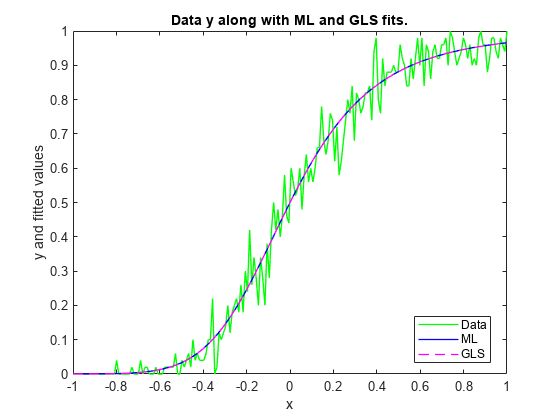
ML and GLS produce similar fitted values.
Plot estimated nonlinear function using ML and GLS
Plot true model for . Add plot for the initial estimate of using and plots for ML and GLS based estimates of .
figure
plot(x,myf(beta,x),'r','LineWidth',1)
hold on
plot(x,myf(beta0,x),'k','LineWidth',1)
plot(x,myf(betaHatML,x),'c--','LineWidth',1)
plot(x,myf(betaHatGLS,x),'b-.','LineWidth',1)
legend('True f','Initial f','Estimated f with ML', ...
    'Estimated f with GLS','Location','Best')
xlabel('x')
ylabel('True and estimated f')
title('Comparison of true f with estimated f using ML and GLS.')
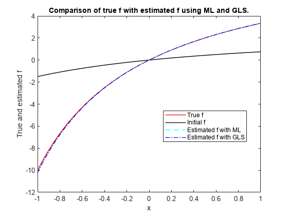
The estimated nonlinear function using both ML and GLS methods is close to the true nonlinear function . You can use a similar technique to fit other nonlinear generalized linear models like nonlinear Poisson regression.