Audio Beamforming on a Multicore Processor

This example shows how to implement an audio beamforming application on a multicore processor. To guarantee that the beamforming algorithms execute in real-time, individual beamforming tasks run on different processor cores.

Algorithm Description

The acoustic beamforming in this example uses a uniform linear array (ULA) of microphones. The application receives three simulated audio signals from different directions on a twenty-element uniformly spaced linear microphone array. After the addition of thermal noise at the receiver, beamforming is applied to each of three different source angles to separate the sources. The image illustrates the application composition.

In this example, the audio sources are simulated by reading the audio samples from binary files. The microphone array and the receiver are also simulated and marked by the red box. The beamformers are the part of the algorithm and they are marked by the green box.

Algorithm Partitioning into Tasks

In this example, the signal generation, the microphone array, and the receiver are simulated, and they are marked as Task1. The model performs three independent beamforming algorithms for each of the expected audio sources. They are marked as Task2, Task3, and Task4.

soc_beamforming_proc;

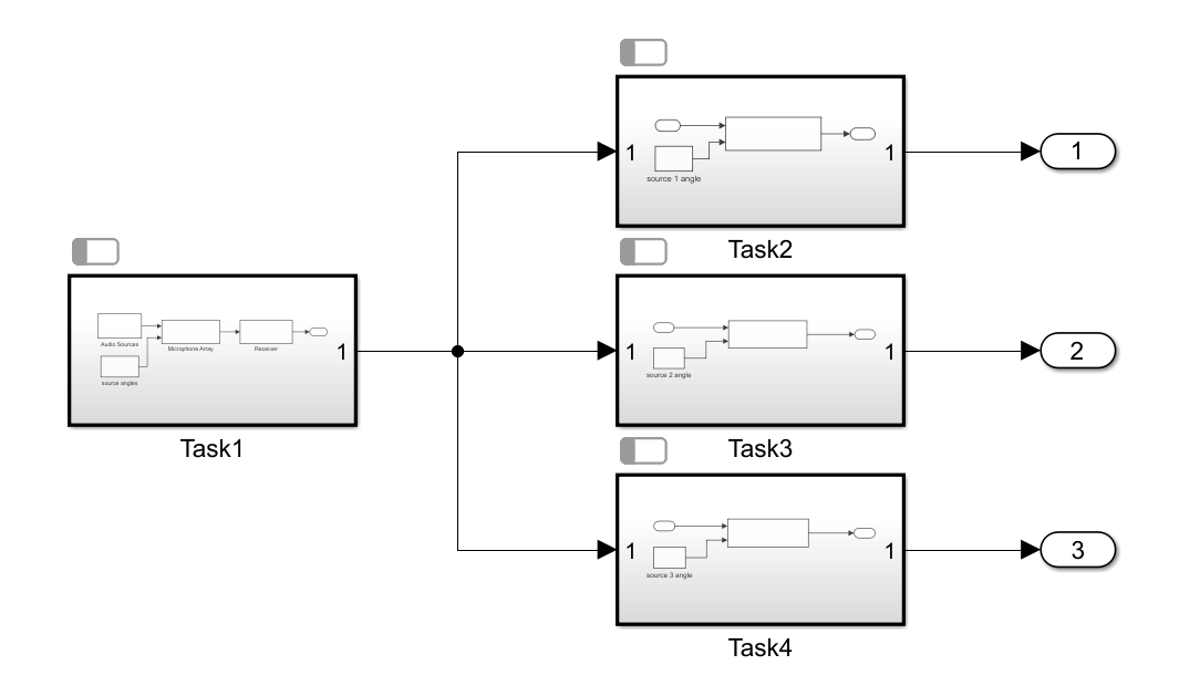
Each task block in this model is created as an explicit periodic task partition, with the period of each partition set to FRAMERATE=FRAMESIZE/SAMPLINGFREQUENCY.

Top Model Description

The task partitions are scheduled for real time execution using the Task Manager block in the top model. The Task Manager blocks sets tasks for each task partition described in the model in the previous step. The tasks are set for the same period as the corresponding partition.

soc_beamforming_top;

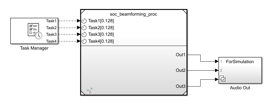
In addition, the top model contains the Audio Out subsystem that has the Audio Device Writer block that plays the audio stream to the computer's audio device in simulation. The Multiport Switch block in the same subsystem allows selecting which of the three audio streams are directed to the audio device.

Simulate the Model

Prepare for Simulation

Three audio source files with different audio recordings are used in this example: soc_dftvoice.wav, soc_cleanvoice.wav, and soc_laughter.wav. The files are provided in the Waveform Audio File format but need to be converted to a binary format so that they can be used both for simulation and for deployed application. Run the provided MATLAB® function to perform the conversion.

soc_beamforming_create_bin;

Three binary files are created as a result: src1.bin, src2.bin, and src3.bin.

Run Simulation

To run the simulation, click Run in the SIMULATION section of the Simulink® toolstrip. Use the Multiport Switch block in the Audio Out subsystem to selecting which audio source to listen to. Change the selected source during the simulation and confirm that the audio stream changes. Observe that there is some interference from other sources, which is expected. The magnitude of the interference depends on the distance among the audio sources.

As it runs, the application writes its outputs to three binary files: output1.bin, output2.bin, and output3.bin. You can play each of these files to an audio device using the following model by entering the file name in the Binary File Reader block.

soc_beamforming_test_output;

You can also analyze the signal spectrum using the Spectrum analyzer block in addition to the Audio Device Writer block. Or you can load the data into MATLAB and perform even more complex analysis, such as correlation.

Deploy the Model to Hardware

Prepare for Deployment

Before running the model on hardware, make sure that you install the SoC Blockset™ Support Package for Xilinx® Devices. The example models are set to Xilinx Zynq® UltraScale+™ RFSoC ZCU111 Evaluation Kit, but you can use any board supported by the support package if it has at least four processor cores. In that case, change the board for all models. Also, run the Setup Hardware app for your board from the HARDWARE BOARD section of the Simulink toolstrip to set up the correct board connection information.

To run the model on hardware, you must set the top model to use the Fixed-step solver. Click the Model Settings in the MODELING section of the Simulink toolstrip and set the Type to Fixed-step in the Solver selection of the Solver page.

To run the model on hardware you also must copy the audio source files you generated to your hardware board. Use the following steps:

Create Connection your Board

Create a connection object to yor board.

hw = socHardwareBoard('Xilinx Zynq UltraScale+ RFSoC ZCU111 Evaluation Kit','hostname','<ipaddress>','username','root','password','root');

If you use a different board, replace the board name with your board name. Also replace <ipaddress> string with your board IP address, which is the same one that you set up earlier via the Setup Hardware app.

Copy Audio Source Files to the Board

Use the connection object hw you created in the previous step to copy the files src1.bin, src2.bin, and src3.bin to your board using the following command in MATLAB for each file.

putFile(hw,'<filename>');

The files will be copied into your home folder on the board. The application will also run in this folder.

Deploy to a Single Core

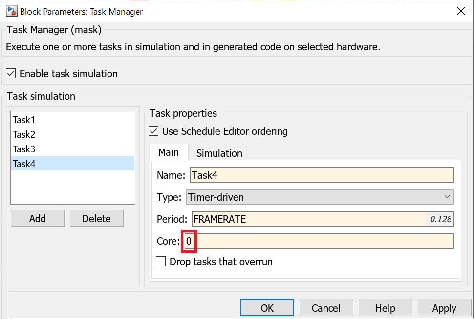
First, run the entire application on a single core. All tasks in the Task Manager block are set to core 0.

For example, Task4 is set to core 0.

Run the model on hardware by clicking the Monitor & Tune in the RUN ON HARDWARE section of the Simulink toolstrip. The model runs in external mode and the execution time statistics are collected for each task.

Analyze the Execution Performance

Click Execution Report in the REVIEW RESULTS section of the Simulink toolstrip to get the summary report.

You can visualize the task execution and the core usage by clicking the Data Inspector in the REVIEW RESULTS section of the Simulink toolstrip. As expected, all tasks run on core 0, one after another.

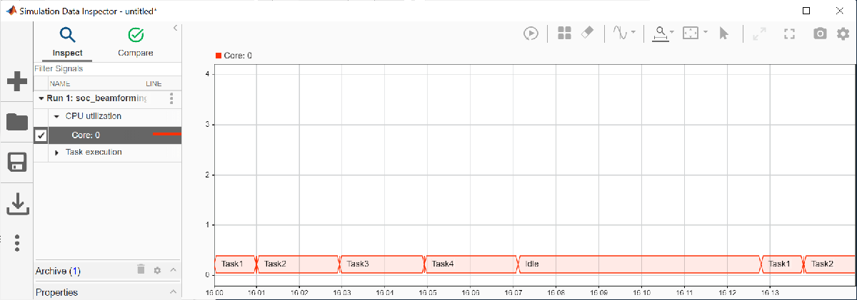
It is evident that running all tasks on one core does not leave a lot of headroom to handle unexpected events and processes in the operating system. Thus, it is advisable to spread the computational burden to other cores.

Verify Application Output

As it runs on hardware, the application writes its outputs to the binary files: output1.bin, output2.bin, and output3.bin. To verify that the application behavior is correct, copy the files from your board to MATLAB for further analysis. Use the same connection object hw you created earlier to copy each file by using the following command in MATLAB.

getFile(hw,'<filename>');

Play each of these files to an audio device using the following model by entering the file name in the Binary File Reader block.

soc_beamforming_test_output;

Deploy to Multiple Cores

Next, run the application on multiple cores. Each task in the Task Manager block is set to a different core.

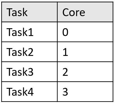
For example, Task4 is set to core 3.

Run the model on hardware by clicking the Monitor & Tune in the RUN ON HARDWARE section of the Simulink toolstrip. The model runs in external mode and the execution time statistics are collected for each task.

Analyze the Execution Performance

Click Execution Report in the REVIEW RESULTS section of the Simulink toolstrip to get the summary report.

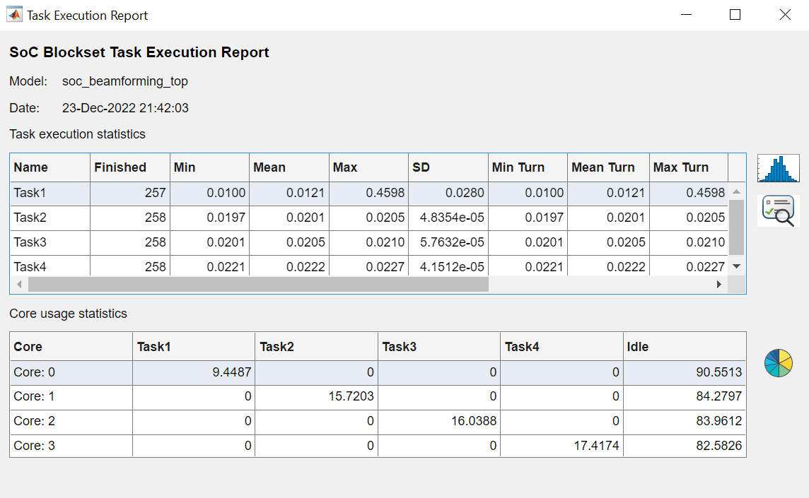
You can visualize the task execution and the core usage by selecting the Data Inspector in the REVIEW RESULTS section of the Simulink toolstrip. All tasks run on different cores concurrently.

You can notice that running tasks on different cores increases the headroom quite substantially and the application is then a lot more robust and able to handle unexpected events and processes in the operating system.

Verify Application Output

As it runs on hardware, the application writes its outputs to the binary files: output1.bin, output2.bin, and output3.bin. To verify that the application behavior is correct, copy the files from your board to MATLAB for further analysis. Use the same connection object hw you created earlier to copy each file by using the following command in MATLAB.

getFile(hw,'<filename>');

Play each of these files to an audio device using the following model by entering the file name in the Binary File Reader block.

soc_beamforming_test_output;

Conclusions

This example showed how to accelerate an algorithm by running it on a multicore processor. By going from one to four cores, the algorithm was accelerated by the factor of ~3.5.

Further Exploration

Change the distance between the audio sources by changing the source angle inputs to the microphone array block and the beamformer blocks. Observe the change in the magnitude of the interference.