Concurrent Execution on Simulink Real-Time
R2026bThis example shows how to apply explicit partitioning to enhance concurrent execution of a real-time application that you generate by using Simulink® Real-Time™.
Simulink Real-Time supports concurrent execution by using implicit partitioning or explicit partitioning of models.
Default Handling of Implicit Partitioning and Tasks
If you do not choose to apply explicit partitioning, Simulink Real-Time applies implicit partitioning to provide concurrent execution of tasks.
For example, consider a multirate Simulink Real-Time model that includes sample times of 50 μs, 1 ms, 10 ms, and 1 s. Implicit partitioning for concurrent execution creates a task for each sample time. By default, when tasks are implicitly scheduled, the task with the smallest sample time (in this case, 50 μs) gets the highest RTOS priority.
In implicit partitioning, shorter sample times are assigned higher task priorities (rate monotonic behavior). This prioritization applies to implicitly scheduled periodic tasks.
You can change the default concurrent execution behavior by applying explicit task partitioning or creating asynchronous tasks. For more information, see the Thread Trigger block.
Explicit Partitioning and Tasks in This Example
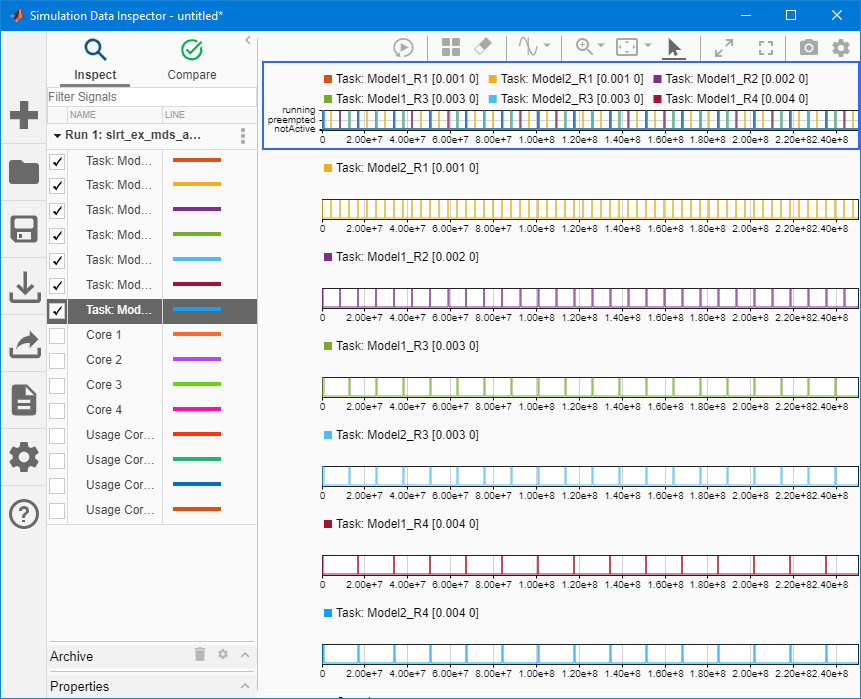
This example shows the relationship between the explicit partitioning of the tasks in the model subsystems and the execution of tasks by using the Simulink Real-Time profiling tool.
Note: You can also use the Simulink® Schedule Editor to partition the model. In the Simulink Editor, click the Modeling tab and select Design > Schedule Editor. For more information, see Create Partitions from a Rate-Based Model.
The example model slrt_ex_mds_and_tasks runs at sample rate of 0.001 second.
To run the model with adjusted sample rate of 0.01 second, change the sample rated before running the example. In the MATLAB® Command Window, type:
Ts = 0.01;
Create Target Object and Connect
Create a Target object for the default target computer and connect to the target computer. In the Command Window, type:
tg = slrealtime;
connect(tg);
Open, Build, and Download the Model
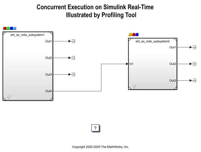
The explicit partitioning in the top-level model occurs in subsystem1.
open_system('slrt_ex_mds_subsystem1');
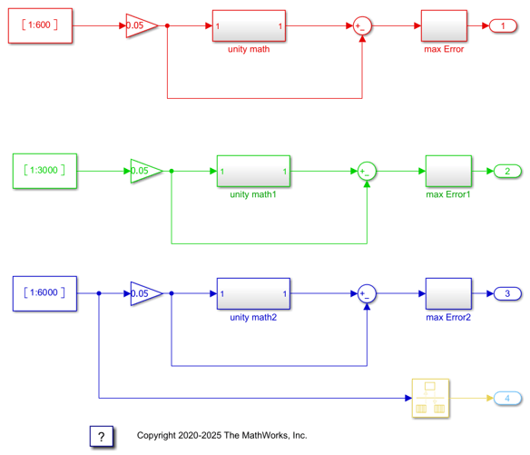
The explicit partitioning in the top-level model occurs in subsystem2.
open_system('slrt_ex_mds_subsystem2');
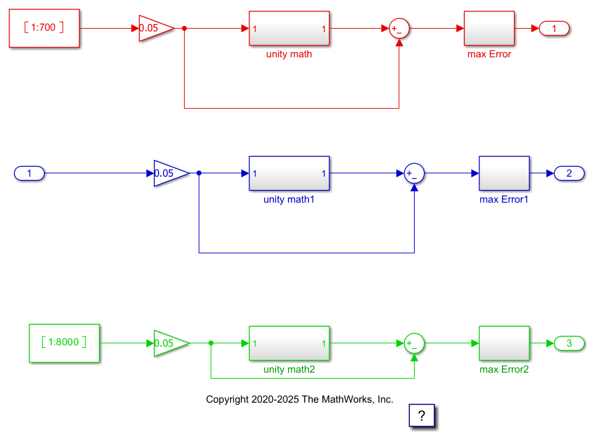
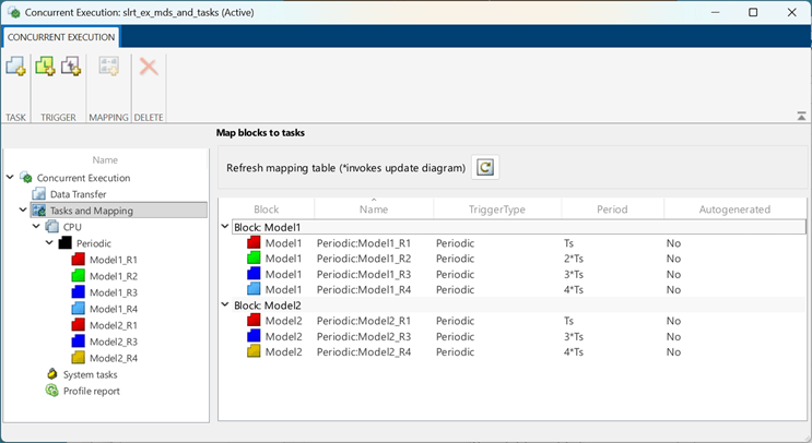
Open the model slrt_ex_mds_and_tasks. The model is mapped to seven threads: Model1_R1, Model1_R2, Model1_R3, Model1_R4, Model2_R1, Model2_R3, and Model2_R4.
These threads run at sample rates of Ts, 2*Ts, 3*Ts, 4*Ts, Ts, 3*Ts, and 4*Ts.
model = 'slrt_ex_mds_and_tasks';
open_system(model);
modelSTF = getSTFName(tg);
set_param(model,"SystemTargetFile",modelSTF);
set_param(model,"StopTime","10");
set_param(model,'RTWVerbose','off');
set_param('slrt_ex_mds_subsystem1',"SystemTargetFile",modelSTF);
set_param('slrt_ex_mds_subsystem2',"SystemTargetFile",modelSTF);
To apply explicit partitioning, in the Simulink Editor, on the Real-Time tab, click Hardware Settings, and then select Solver > Configure Tasks. Select the Tasks and Mapping node. For more information, see Configure Your Model for Concurrent Execution and Concurrent Execution.
Build, download, and run the model.
evalc('slbuild(model)');
load(tg,model);
Open TET Monitor
slrtTETMonitor;
Start application and profile the application on the target computer
startProfiler(tg);
start(tg);
pause(2);
stopProfiler(tg);
stop(tg);
Display Profiling Data
The profiling data shows the execution time of each thread on a multi-core target computer.
getProfilerData(tg,model,"slrt_ex_mds_and_tasks_profiler_data");
Processing data on target computer ...
View TET Information in TET monitor

View TET Information in the Simulation Data Inspector
See Also
For more information, see:
Close the Model
bdclose('slrt_ex_mds_subsystem1');
bdclose('slrt_ex_mds_subsystem2');
bdclose(model);
See Also
stopProfiler | startProfiler | resetProfiler | getProfilerData | getAvailableProfile | deleteProfilerData

