Fixed Step Solvers in Simulink

Fixed-step solvers solve the model at regular time intervals from the beginning to the end of the simulation. The size of the interval is known as the step size. You can specify the step size or let the solver choose the step size. Generally, a smaller the step size increases the accuracy of the results but also increases the time required to simulate the system.

Fixed-Step Discrete Solver

The fixed-step discrete solver computes the time of the next simulation step by adding a fixed step size to the current time. The accuracy and the length of time of the resulting simulation depends on the size of the steps taken by the simulation: the smaller the step size, the more accurate the results are but the longer the simulation takes. By default, Simulink^® chooses the step size or you can choose the step size yourself. If you choose the default setting of auto, and if the model has discrete sample times, then Simulink sets the step size to the fundamental sample time of the model. Otherwise, if no discrete rates exist, Simulink sets the size to the result of dividing the difference between the simulation start and stop times by 50.

Fixed-Step Continuous Solvers

The fixed-step continuous solvers, like the fixed-step discrete solver, compute the next simulation time by adding a fixed-size time step to the current time. For each of these steps, the continuous solvers use numerical integration to compute the values of the continuous states for the model. These values are calculated using the continuous states at the previous time step and the state derivatives at intermediate points (minor steps) between the current and the previous time step.

Note

Simulink uses the fixed-step discrete solver for a model that contains no states or only discrete states, even if you specify a fixed-step continuous solver for the model.

Simulink provides two types of fixed-step continuous solvers — explicit and implicit.

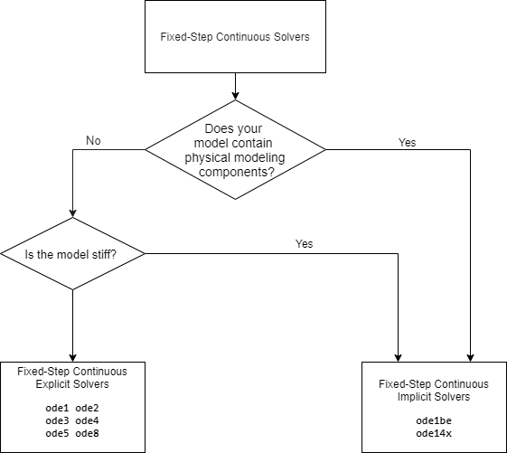
The difference between these two types lies in the speed and the stability. An implicit solver requires more computation per step than an explicit solver but is more stable. Therefore, the implicit fixed-step solver that Simulink provides is more adept at solving a stiff system than the fixed-step explicit solvers. For a comparison of explicit and implicit solvers, see Explicit Versus Implicit Continuous Solvers.

Fixed-Step Continuous Explicit Solvers

Explicit solvers compute the value of a state at the next time step as an explicit function of the current values of both the state and the state derivative. A fixed-step explicit solver is expressed mathematically as:

$$x(n+1)=x(n)+h\ast Dx(n)$$

where

• x is the state.

• Dx is a solver-dependent function that estimates the state derivative.

• h is the step size.

• n indicates the current time step.

Simulink provides a set of fixed-step continuous explicit solvers. The solvers differ in the specific numerical integration technique that they use to compute the state derivatives of the model. This table lists each solver and the integration technique it uses. The table lists the solvers in the order of the computational complexity of the integration methods they use, from the least complex (ode1) to the most complex (ode8).

Solver	Integration Technique	Order of Accuracy
ode1	Euler's method	First
ode2	Heun's method	Second
ode3	Bogacki-Shampine formula	Third
ode4	Fourth-order Runge-Kutta (RK4) formula	Fourth
ode5	Dormand-Prince (RK5) formula	Fifth
ode8	Dormand-Prince RK8(7) formula	Eighth

None of these solvers have an error control mechanism. Therefore, the accuracy and the duration of a simulation depend directly on the size of the steps taken by the solver. As you decrease the step size, the results become more accurate, but the simulation takes longer. Also, for any given step size, the higher the order of the solver, the more accurate the simulation results.

If you specify a fixed-step solver type for a model, then by default, Simulink selects the FixedStepAuto solver. Auto solver then selects an appropriate fixed-step solver that can handle both continuous and discrete states with moderate computational effort. As with the discrete solver, if the model has discrete rates (sample times), then Simulink sets the step size to the fundamental sample time of the model by default. If the model has no discrete rates, Simulink automatically uses the result of dividing the simulation total duration by 50. Consequently, the solver takes a step at each simulation time at which Simulink must update the discrete states of the model at its specified sample rates. However, it does not guarantee that the default solver accurately computes the continuous states of a model. Therefore, you may need to choose another solver, a different fixed step size, or both to achieve acceptable accuracy and an acceptable simulation time.

Fixed-Step Continuous Implicit Solvers

An implicit solver computes the state at the next time step as an implicit function of the state at the current time step and the state derivative at the next time step, as described by the following expression.

$$x(n+1)-x(n)-h\ast Dx(n+1)=0$$

Simulink provides two fixed-step implicit solvers: ode14x and ode1be. This solver uses a combination of Newton's method and extrapolation from the current value to compute the value of a state at the next time step. You can specify the number of Newton's method iterations and the extrapolation order that the solver uses to compute the next value of a model state. See Fixed-step size (fundamental sample time). The more iterations and the higher the extrapolation order that you select, the greater the accuracy you obtain. However, you simultaneously create a greater computational burden per step size.