Calculate Optical Flow by Using Neighborhood Processing Subsystem Blocks
This example shows how to calculate optical flow in a video by using Neighborhood Processing Subsystem blocks. Optical flow is the distribution of the apparent velocities of objects in an image. Use optical flow to identify and track objects in a video.
Inspect Model
Open the model.
model = 'OpticalFlowNeighborhoodExample';
open_system(model);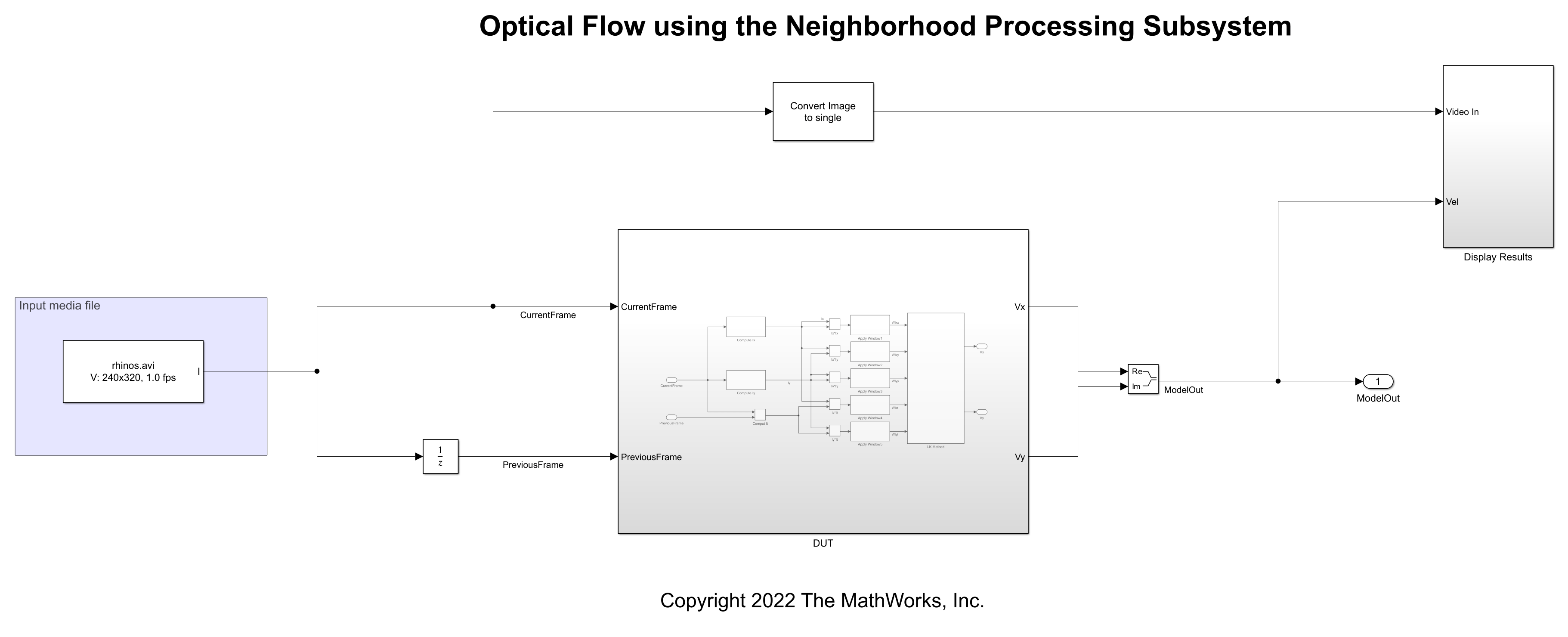
The model references a video input, rhinos.avi, by using the From Multimedia File (Computer Vision Toolbox) block. At each iteration, the model passes the current and previous frames of the video to the DUT subsystem, which performs the optical flow calculation. This calculation outputs an optical flow matrix which represents the apparent motion at each pixel of the video. The model overlays these calculated motion vectors over the input video.
Open the DUT subsystem.
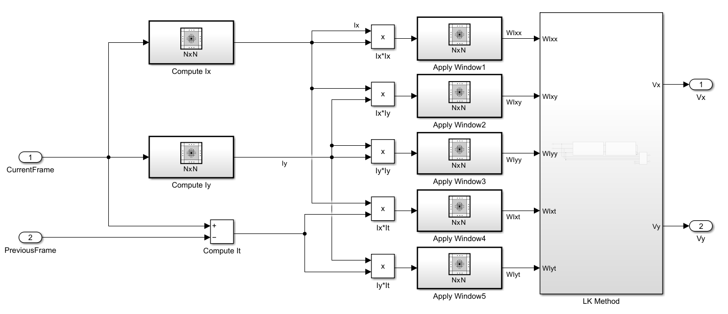
This example calculates optical flow by using the Lucas-Kanade method. The Lucas-Kanade method requires the values , , and , which are the derivatives of pixel brightness along the horizontal direction, vertical direction, and time, respectively.
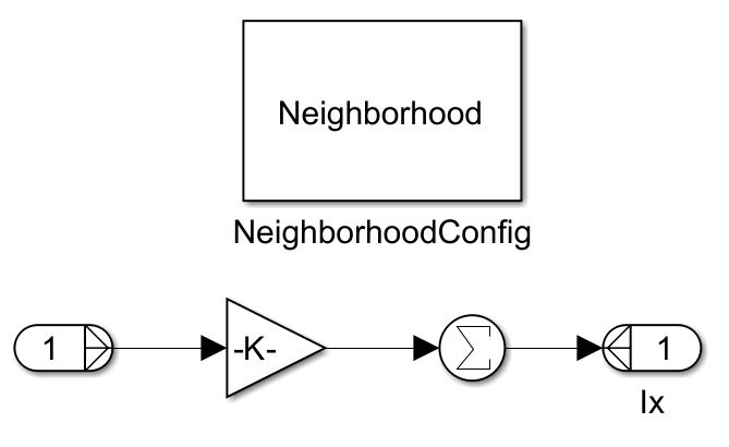
The Compute Ix Neighborhood Processing Subsystem block calculates by using a 1-by-5 neighborhood and these blocks. The Neighborhood control block NeighborhoodConfig specifies the neighborhood size using its Neighborhood size parameter.
The Compute Iy subsystem calculates with the same blocks and a 5-by-1 neighborhood. The model calculates as the difference between the current video frame and previous video frame by using a Sum block.
The horizontal optical flow and vertical optical flow represent the solution to this equation.
To solve this equation, the Lucas-Kanade method divides the input image into smaller sections and assumes a constant velocity in each section. Then it performs a weighted, least-square fit of the optical flow constraint equation to a constant model for in each section . The method achieves this fit by minimizing this equation, where is a window function that emphasizes the constraints at the center of each section:
The solution to the minimization problem is:
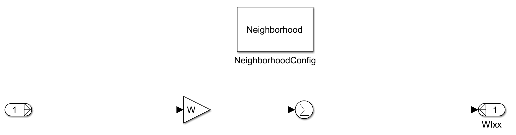
The example calculates , , , and by using Product blocks. The example implements by using Neighborhood Processing Subsystem blocks with 5-by-5 neighborhoods.
Open the LK Method subsystem.
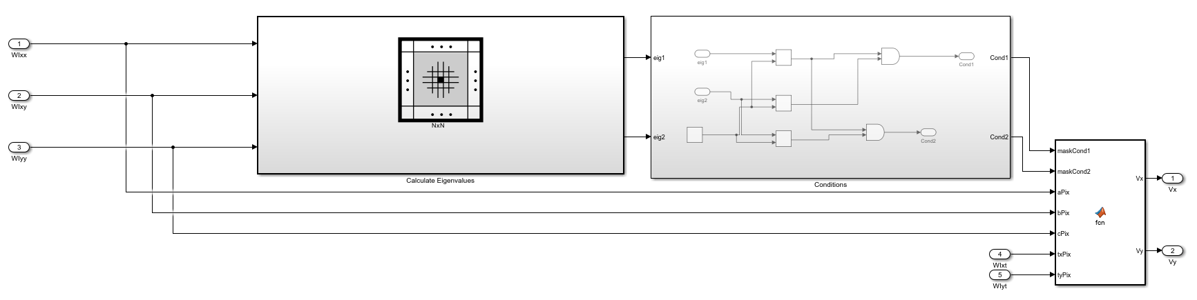
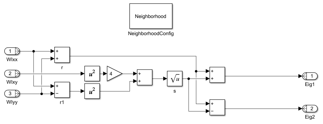
The Calculate Eigenvalues Neighborhood Processing Subsystem block calculates the eigenvalues of by solving the equation .
The example implements the rest of the Lucas-Kanade method by using the Conditions subsystem and a MATLAB Function block. For information about these calculations, see opticalFlowLK (Computer Vision Toolbox).
Simulation and Results
Simulate the model. The model displays the input video with vectors overlaid, representing the optical flow.

Close the model.
close_system(model);
See Also
Neighborhood
Processing Subsystem | Optical Flow (Computer Vision Toolbox) | opticalFlowLK (Computer Vision Toolbox)
Topics
- Stabilize Video Using Optical Flow (Computer Vision Toolbox)
- Perform Edge Detection by Using a Neighborhood Processing Subsystem Block
- Perform Corner Detection by Using Neighborhood Processing Subsystem Blocks
- Generate HDL Code from Frame-Based Models by Using Neighborhood Modeling Methods (HDL Coder)
- Use Neighborhood, Reduction, and Iterator Patterns with a Frame-Based Model or Function for HDL Code Generation (HDL Coder)