Robust Stability and Worst-Case Gain of Uncertain System

This example shows how to calculate the robust stability and examine the worst-case gain of the closed-loop system described in System with Uncertain Parameters. The following commands construct that system.

m1 = ureal('m1',1,'percent',20);
m2 = ureal('m2',1,'percent',20);
k  = ureal('k',1,'percent',20);

s = zpk('s'); 
G1 = ss(1/s^2)/m1; 
G2 = ss(1/s^2)/m2; 


F = [0;G1]*[1 -1]+[1;-1]*[0,G2];
P = lft(F,k); 

C = 100*ss((s+1)/(.001*s+1))^3;

T = feedback(P*C,1); % Closed-loop uncertain system

This uncertain state-space model T has three uncertain parameters, k, m1, and m2, each equal to 1±20% uncertain variation. Use robstab to analyze whether the closed-loop system T is robustly stable for all combinations of possible values of these three parameters.

[stabmarg,wcus] = robstab(T);
stabmarg

stabmarg = struct with fields:
           LowerBound: 2.8819
           UpperBound: 2.8864
    CriticalFrequency: 575.0339

The data in the structure stabmarg includes bounds on the stability margin, which indicate that the control system can tolerate almost 3 times the specified uncertainty before going unstable. It is stable for all parameter variations in the specified ±20% range. The critical frequency is the frequency at which the system is closest to instability.

The structure wcus contains the smallest destabilization perturbation values for each uncertain element.

wcus

wcus = struct with fields:
     k: 1.5773
    m1: 0.4227
    m2: 0.4227

You can evaluate the uncertain model at these perturbation values using usubs. Examine the pole locations of that worst-case model.

Tunst = usubs(T,wcus);   
damp(Tunst)

                                                                       
         Pole              Damping       Frequency      Time Constant  
                                       (rad/seconds)      (seconds)    
                                                                       
 -8.82e-01 + 1.55e-01i     9.85e-01       8.95e-01         1.13e+00    
 -8.82e-01 - 1.55e-01i     9.85e-01       8.95e-01         1.13e+00    
 -1.25e+00                 1.00e+00       1.25e+00         7.99e-01    
  2.02e-06 + 5.75e+02i    -3.52e-09       5.75e+02        -4.95e+05    
  2.02e-06 - 5.75e+02i    -3.52e-09       5.75e+02        -4.95e+05    
 -1.50e+03 + 6.44e+02i     9.19e-01       1.63e+03         6.67e-04    
 -1.50e+03 - 6.44e+02i     9.19e-01       1.63e+03         6.67e-04    

The system contains a pair of poles very close to the imaginary axis, with a damping ratio of less than 1e-7. This result confirms that the worst-case perturbation is just enough to destabilize the system.

Use wcgain to calculate the worst-case peak gain, the highest peak gain occurring within the specified uncertainty ranges.

[wcg,wcug] = wcgain(T);
wcg

wcg = struct with fields:
           LowerBound: 1.0471
           UpperBound: 1.0731
    CriticalFrequency: 7.7158

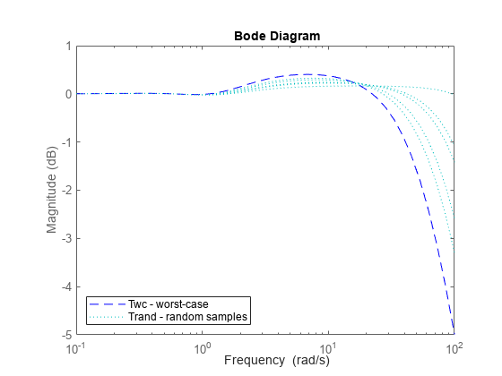
wcug contains the values of the uncertain elements that cause the worst-case gain. Compute a closed-loop model with these values, and plot its frequency response along with some random samples of the uncertain system.

Twc = usubs(T,wcug); 
Trand = usample(T,5); 
bodemag(Twc,'b--',Trand,'c:',{.1,100});
legend('Twc - worst-case','Trand - random samples','Location','SouthWest');

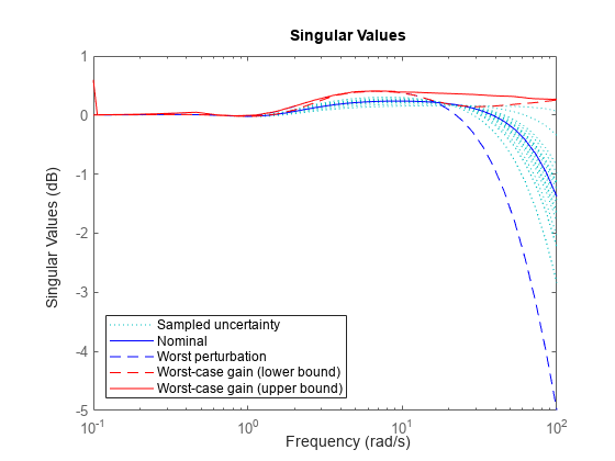
Alternatively use wcsigmaplot to visualize the highest possible gain at each frequency, the system with the highest peak gain, and random samples of the uncertain system.

wcsigmaplot(T,{.1,100})