Lossy Multiconductor Transmission Line Circuit
This example shows how to analyze a lossy multiconductor transmission line circuit. The transmission lines are modeled using RLGC distributed elements which are used in signal integrity analysis for accurately capturing high-speed interconnect effects. You can analyze this circuit using RF Toolbox™ pwlresp function or using RF Blockset™ Circuit Envelope model. In this example you first compute the time-domain response of the circuit excited by a periodic pulse signal and then you compare the result to a circuit simulated using the RF Blockset Circuit Envelope simulation.
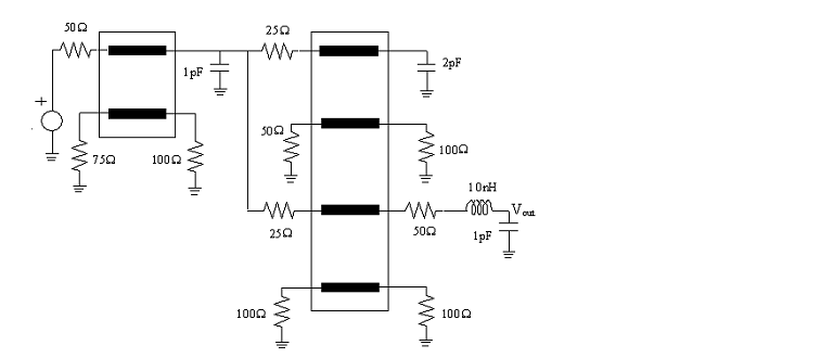
Figure 1: Interconnect circuit with lossy multiconductor transmission lines
Representation of Distributed Transmission Line Models with N-Port Elements
The circuit in this example contains two sets of lossy coupled transmission lines. The RLGC line parameter matrices of the two lines are as follows [1].
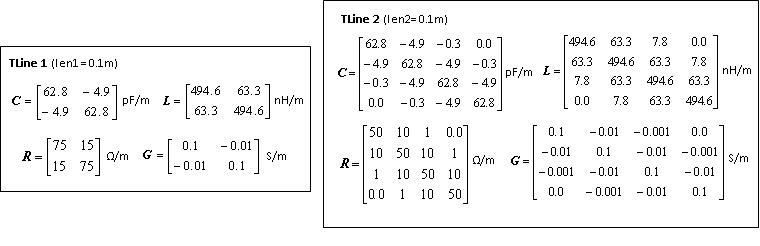
Figure 2: RLGC line parameters for the 4-ports and 8-ports transmission lines
Extract the S-parameters of each coupled transmission lines using rlgc2s function. Then represent the S-parameters using an nport element.
freq = linspace(1e1,8e9,1001);
N = length(freq);
len1 = 0.1;
R1 = ones(2,2,N).*[75,15;15,75];
L1 = ones(2,2,N).*[494.6,63.3;63.3,494.6]*1e-9;
G1 = ones(2,2,N).*[0.1,-0.01;-0.01,0.1];
C1 = ones(2,2,N).*[62.8,-4.9;-4.9,62.8]*1e-12;

s_params1 = rlgc2s(R1,L1,G1,C1,len1,freq);
stlobj1 = sparameters(s_params1,freq);
nport_s1 = nport(stlobj1);

len2 = 0.1;
R2 = ones(4,4,N).*[50,10,1,0.0;10,50,10,1;1,10,50,10;0.0,1,10,50];
L2 = ones(4,4,N).*[494.6,63.3,7.8,0.0;63.3,494.6,63.3,7.8;7.8,63.3,494.6,63.3;0.0,7.8,63.3,494.6]*1e-9;
G2 = ones(4,4,N).*[0.1,-0.01,-0.001,0.0;-0.01,0.1,-0.01,-0.001;-0.001,-0.01,0.1,-0.01;0.0,-0.001,-0.01,0.1];
C2 = ones(4,4,N).*[62.8,-4.9,-0.3,0.0;-4.9,62.8,-4.9,-0.3;-0.3,-4.9,62.8,-4.9;0.0,-0.3,-4.9,62.8]*1e-12;

s_params2 = rlgc2s(R2,L2,G2,C2,len2,freq);
stlobj2 = sparameters(s_params2,freq);
nport_s2 = nport(stlobj2);
Calculation of S-Parameter Object of Interconnect Circuit
Calculate the S-parameter object of the circuit given in Figure.1 by using the sparameters function.
ckt = circuit('interconnect');

add(ckt,[1 2],resistor(50))
add(ckt,[2 3 4 5],nport_s1,{'p1+' 'p2+' 'p3+' 'p4+'})
add(ckt,[3 0],resistor(75))
add(ckt,[4 0],capacitor(1e-12))
add(ckt,[5 0],resistor(100))
add(ckt,[4 6],resistor(25))
add(ckt,[7 0],resistor(50))
add(ckt,[4 8],resistor(25))
add(ckt,[9 0],resistor(100))
add(ckt,[6 7 8 9 10 11 12 13],nport_s2,{'p1+' 'p2+' 'p3+' 'p4+' 'p5+' 'p6+' 'p7+' 'p8+'})
add(ckt,[10 0],capacitor(2e-12))
add(ckt,[11 0],resistor(100))
add(ckt,[13 0],resistor(100))
add(ckt,[12 14],resistor(50))
add(ckt,[14 15],inductor(10e-9))
add(ckt,[15 0],capacitor(1e-12))

freqfit = linspace(1e1,8e9,1001)';
setports(ckt,[1 0],[15 0])
S_vout = sparameters(ckt,freqfit);
Generation of Rational Object of Multiconductor Transmission Line Circuit
Convert the transfer function of the S-parameter object of the circuit to a rational object over the specified frequencies. Then calculate the frequency response using the freqresp function.
tfblkout = s2tf(S_vout,0,Inf,2);
fitblkout = rational(freqfit,tfblkout);

plot(freqfit/1e9,abs(tfblkout),'b',freqfit/1e9,abs(freqresp(fitblkout,freqfit)),'r:','LineWidth',2)
legend('Original data','Fitting result')
title('Frequency Response')
ylabel('Magnitude')
xlabel('Frequency (GHz)')
![]()
Computation of Transient Waveform Excited by Periodic Pulse Source
Apply a voltage source using a 1 V periodic pulse with a rise/fall time of 0.4 ns, a duration of 5 ns, and a period of 1.6 ns. Then compute the time-domain response of the circuit by using the pwlresp function.
SignalTime = [0,0.4,5.4,5.8]*1e-9;
SignalValue = [0,1,1,0];
Tsim = (0:1e-11:6e-8);
TP = 1.6e-8;
[WAVEOUT, tout] = pwlresp(fitblkout,SignalTime,SignalValue,Tsim,TP);

plot(tout,WAVEOUT, 'LineWidth',2)
legend('PWLRESP')
title('Output Waveform')
xlabel('Time (s)')
ylabel('Output (V)')
ylim([-0.05 0.38])
![]()
Comparison of Time-Domain Response of Coupled Transmission Line Circuit Using RF Blockset
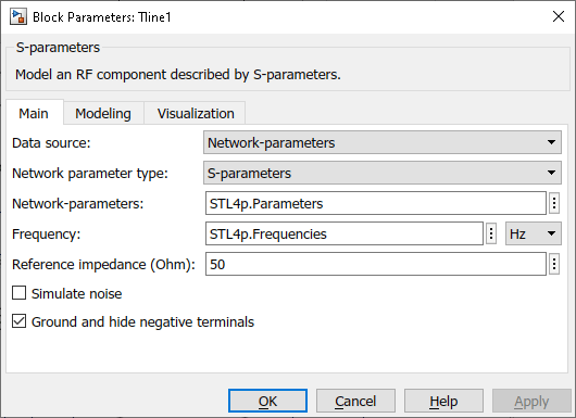
A Simulink model is built to simulate the multiconductor transmission line circuit shown in Figure 1. With the S-parameters calculated from previous session, the multiconductor transmission lines can be represented by S-parameter blocks from RF Blockset Circuit Envelope Library. For instance, the 4-port transmission lines are modeled by defining the S-parameter block mask as shown below, where STL4p is a S-parameter object converted from reordering ports of S-parameter object stlobj1 with snp2smp function. The output of the model is the time-domain response in the form of a passband signal. For more information on passband signal implementation in the Circuit Envelope model, see Passband Signal Representation in Circuit Envelope (RF Blockset).
To simulate the model:
Type
open_system('simrf_coupled_pb')at the command prompt.Select Simulation > Run.
After you finish simulating the model, compare the obtained transient waveform with that calculated using RF Toolbox.
open_system('simrf_coupled_pb');
sim('simrf_coupled_pb');
plot(tout,WAVEOUT,CE_Data(:,1),CE_Data(:,2),'--','LineWidth',2)
legend('PWLRESP', 'Circuit Envelope')
title('Time-Domain Response of Lossy Coupled Transmission Lines')
xlabel('Time (s)')
ylabel('Output (V)')
ylim([-0.05 0.38])
![]()
![]()
bdclose('simrf_coupled_pb');
References
[1] Tang, Tak K., and Michel Nakhla. “Analysis of High-Speed VLSI Interconnects Using the Asymptotic Waveform Evaluation Technique.” IEEE Transactions on Computer-Aided Design of Integrated Circuits and Systems 11, no. 3 (March 1992): 341–52. https://doi.org/10.1109/43.124421.