Create Custom Vectorized Environment Functions from Template

R2026b

This example shows how to scaffold a vectorized reinforcement learning environment using a template file provided as a helper function in this directory. Specifically, the example walks you through generating a vectorized environment from the template, customizing the functions to model a simple mass-spring-damper system, and simulating the system against a pre-tuned linear policy.

Define Observation and Action Specifications

The environment has a 2-element state vector $${\left[x,\underset{}{\overset{\dot{}}{x}}\right]}^T$$in which the first element represents displacement and the second element represents velocity. The action represents a bounded scalar force $$F\in \left[-1,1\right]$$ applied directly to the mass.

obsInfo = rlNumericSpec([2 1]);
obsInfo.Name = "obs";

actInfo = rlNumericSpec([1 1], ...
    UpperLimit= 1, ...
    LowerLimit=-1);
actInfo.Name = "force";

Generate Template Environment Functions

Use generateFunctionVectorEnvFromTemplate, which is attached to this example as a supporting file, to create the four function files that define a vectorized environment: a factory function, a setup function, a reset function, and a step function. Use the StateSpec name-value argument to define the state data structure for the environment in the template functions. The first argument you provide to generateFunctionVectorEnvFromTemplate specifies the naming convention for the generated functions.

generateFunctionVectorEnvFromTemplate("mass_spring_venv", ...
    obsInfo, actInfo, ...
    StateSpec=rlNumericSpec([2 1],Name="State"));

Inspect the generated setup function. This function sets up environment instances for the vectorized environment.

type mass_spring_venv_setup.m

function env_data = mass_spring_venv_setup(info)
% Setup environment instances for mass_spring_venv.

% Generated on 06-Aug-2026 23:51:21 with generateFunctionVectorEnvFromTemplate

env_data.State = zeros(2, 1, info.NumEnv);

Inspect the generated reset function. This function resets the vectorized environment instances.

type mass_spring_venv_reset.m

function [obs, env_data] = mass_spring_venv_reset(env_data, resetidx)
% Reset environment instances for mass_spring_venv.

% Generated on 06-Aug-2026 23:51:21 with generateFunctionVectorEnvFromTemplate.

num_env = numel(resetidx);
num_reset_env = nnz(resetidx);

% Reset state for indicated instances.
env_data.State(:, :, resetidx) = 0;
x = env_data.State;

% Form observation from state.
obs{1} = zeros(2, 1, num_reset_env);

Inspect the generated step function. This function steps the vectorized environment instances.

type mass_spring_venv_step.m

function [obs, rwd, isd, env_data] = mass_spring_venv_step(env_data, act)
% Step environment instances for mass_spring_venv.

% Generated on 06-Aug-2026 23:51:21 with generateFunctionVectorEnvFromTemplate.

num_env = size(act{1}, 3);
act = act{1};
x = env_data.State;

% Implement environment dynamics.
% x = ...

% Compute reward.
rwd = zeros(1, num_env);

% Form observation from state.
obs{1} = zeros(2, 1, num_env);

% Compute termination condition.
isd = zeros(1, num_env, "uint8");

% Store the updated state.
env_data.State = x;

Inspect the generated factory function. This function constructs the rlFunctionVectorEnv object from the environment functions.

type mass_spring_venv.m

function venv = mass_spring_venv(args)
% Create mass_spring_venv vectorized environment.

% Generated on 06-Aug-2026 23:51:21 with generateFunctionVectorEnvFromTemplate.

arguments
	args.?rl.venv.rlVectorEnv
end

oinfo = rlNumericSpec([2 1], ...
    UpperLimit=Inf, ...
    LowerLimit=-Inf);
oinfo.Name = "obs";

ainfo = rlNumericSpec([1 1], ...
    UpperLimit=1, ...
    LowerLimit=-1);
ainfo.Name = "force";

venv = rlFunctionVectorEnv(oinfo, ainfo, ...
	@mass_spring_venv_step, ...
	@mass_spring_venv_reset, ...
	@mass_spring_venv_setup);

fs = fieldnames(args);
for i = 1:numel(fs)
	f = fs{i};
	venv.(f) = args.(f);
end

Customize the Generated Functions

In the generated files, you can modify the commands that calculate the dynamics, reset behavior, and setup behavior of your environment.

For this example, to customize the setup, reset, and step functions, replace the generated template files with a pre-made implementation of the mass-spring-damper dynamics with force applied at the mass. Specifically, the new setup, reset, and step functions implement the system with the following dynamics:

$$m\underset{}{\overset{¨}{x}}+c\underset{}{\overset{\dot{}}{x}}+kx=F$$

with parameters $$m=1$$(mass), $$k=1$$ (spring force), $$c=0.1$$ (damping coefficient), using the SI unit system. The integration timestep is $$\Delta t=0.05$$ seconds. The reward is $$r=-\left|x\right|$$, and episodes terminate when $$\left|x\right|>2$$.

copyfile("supportingFiles/mass_spring_venv_setup.m", "mass_spring_venv_setup.m")
copyfile("supportingFiles/mass_spring_venv_reset.m", "mass_spring_venv_reset.m")
copyfile("supportingFiles/mass_spring_venv_step.m" , "mass_spring_venv_step.m" )

Inspect the modified setup function.

type mass_spring_venv_setup.m

function env_data = mass_spring_venv_setup(info)
% Setup environment instances for mass_spring_venv.

% Generated with generateFunctionVectorEnvFromTemplate

env_data.State = zeros(2, 1, info.NumEnv);

% Physical parameters.
env_data.m  = 1.0;    % mass (kg)
env_data.k  = 1.0;    % spring stiffness (N/m)
env_data.c  = 0.1;    % damping coefficient (Ns/m)
env_data.dt = 0.05;   % integration timestep (s)

Inspect the modified reset function.

type mass_spring_venv_reset.m

function [obs, env_data] = mass_spring_venv_reset(env_data, resetidx)
% Reset environment instances for mass_spring_venv.

% Generated with generateFunctionVectorEnvFromTemplate.

num_reset_env = nnz(resetidx);

% Reset state for indicated instances.
% Randomize initial conditions from Uniform(-1, 1).
env_data.State(:, :, resetidx) = 2*rand(2, 1, num_reset_env) - 1;
x = env_data.State;

% Form observation from state.
obs{1} = x(:, :, resetidx);

Inspect the modified step function.

type mass_spring_venv_step.m

function [obs, rwd, isd, env_data] = mass_spring_venv_step(env_data, act)
% Step environment instances for mass_spring_venv.

% Generated with generateFunctionVectorEnvFromTemplate.

% Extract action and state.
F = max(min(act{1}, 1.0), -1.0);
num_env = size(F, 3);
x = env_data.State;

% Extract state components.
pos  = x(1, 1, :);
vel  = x(2, 1, :);

% Physical parameters.
m  = env_data.m;
k  = env_data.k;
c  = env_data.c;
dt = env_data.dt;

% Implement environment dynamics.
% Forward Euler integration of mass-spring-damper: m*xddot + c*xdot + k*x = F
xddot = (F - c.*vel - k.*pos) ./ m;
vel   = vel + dt.*xddot;
pos   = pos + dt.*vel;

% Compute reward.
rwd = reshape(-abs(pos), 1, num_env);

% Form observation from state.
x(1, 1, :) = pos;
x(2, 1, :) = vel;
obs{1} = x;

% Compute termination condition.
isd = reshape(uint8(abs(pos) > 2), 1, num_env);

% Store the updated state.
env_data.State = x;

Create the Vectorized Environment

Call the factory function to construct the vectorized mas-spring-damper environment with 64 parallel instances.

venv = mass_spring_venv(NumEnv=64);

Now that the vectorized environment is created, you can use it to train a reinforcement learning agent. For this example, instead of training an agent, use the rollout function to simulate the vectorized environment against a linear policy that represents a proportional-derivative (PD) controller.

Define a Linear PD Controller Policy

Express a PD controller as a linear policy $$F=\left[-k_p-k_d\right]{\left[x,\underset{}{\overset{\dot{}}{x}}\right]}^T$$ with pre-tuned gains. Use rlContinuousDeterministicActor to create a continuous deterministic actor object using a linear basis function as underlying approximation model. The first input argument is a two-element cell array. The first element of the cell array is the handle to a custom basis function which simply returns the input vector s. The second element of the cell array is the vector of initial learnable parameters -[kp kd]'. The output of the actor is the inner product between the learnable parameter vector, (which in this example does not change because you only simulate the actor, but do not train it), and the basis function output s.

kp = 5.0;
kd = 4.0;
actor = rlContinuousDeterministicActor({@(s) s, -[kp kd]'}, obsInfo, actInfo);
policy = rlDeterministicActorPolicy(actor);

Run Vectorized Rollout

Use rollout to simulate 100 steps across all 64 environment instances simultaneously.

numSteps = 100;
[nobs, obs, act, rwd] = rollout(venv, policy, numSteps, MaxStepsPerEpisode=numSteps);

Plot Trajectories From Each Environment Instance

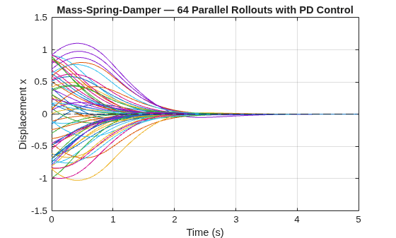
To form the full observation trajectory, concatenate the initial observations with the next observations. Extract the displacement $$x$$ from each environment instance and overlay all trajectories on the same plot. The plot shows the PD controller regulating the mass back to equilibrium from each initial displacement.

% Reshape the current and next observations.
obs_shaped  = reshape( obs{1}, 2, [], venv.NumEnv);
nobs_shaped = reshape(nobs{1}, 2, [], venv.NumEnv);

% Concatenate the initial observations with the next observations.
obs_traj = [obs_shaped(:,1,:), nobs_shaped];
pos = squeeze(obs_traj(1,:,:));

% Time vector
dt = 0.05;
t = (0:numSteps)*dt;

% Plot
figure;
plot(t,pos);
yline(0, "--k");
xlabel("Time (s)");
ylabel("Displacement x");
title("Mass-Spring-Damper — 64 Parallel Rollouts with PD Control");
grid on;

Extract the applied force and per-step reward from the rollout to view the control effort and performance across all environment instances.

F   = squeeze(reshape(act{1}, 1, [], venv.NumEnv)); % [numSteps, NumEnv]
rwd = squeeze(reshape(rwd   , 1, [], venv.NumEnv)); % [numSteps, NumEnv]

% Plot
figure;
tiledlayout(2, 1);
t = (0:(numSteps-1))*dt;

nexttile;
plot(t, F);
yline(0, "--k");
xlabel("Time (s)");
ylabel("Force F");
title("Applied Control Force");
grid on;

nexttile;
plot(t, rwd);
yline(0, "--k");
xlabel("Time (s)");
ylabel("Reward");
title("Reward (r = -|x|)");
grid on;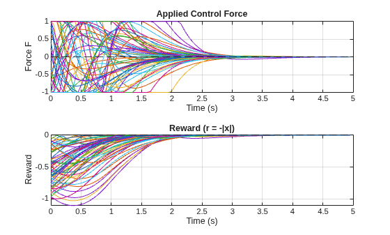

The control force decays as the mass approaches equilibrium, and the reward increases toward zero as displacement diminishes.