진동 신호를 사용한 상태 모니터링 및 예지진단

라이브 스크립트 열기

이 예제에서는 볼 베어링의 진동 신호에서 특징을 추출하고, 건전성 모니터링을 실시하고, 예지진단을 수행하는 방법을 보여줍니다. 이 예제에서는 Signal Processing Toolbox™ 및 System Identification Toolbox™의 기능을 사용하며, Predictive Maintenance Toolbox™는 필요하지 않습니다.

데이터 설명

pdmBearingConditionMonitoringData.mat 에 저장된 진동 데이터를 불러옵니다(MathWorks 지원 파일 사이트에서 다운로드한 최대 88MB의 대규모 데이터셋). 데이터는 셀형 배열에 저장되어 있으며, 이는 베어링 외륜에 단일 결함이 있는 볼 베어링 신호 시뮬레이터를 사용하여 생성되었습니다. 데이터는 여러 건전성 상태에서 시뮬레이션된 베어링에 대한 진동 신호의 여러 세그먼트를 포함합니다(결함 깊이는 3um에서 3mm 이상까지로 증가함). 각 세그먼트는 샘플링 레이트 20kHz로 1초 동안 수집한 신호를 저장합니다. pdmBearingConditionMonitoringData.mat에서 defectDepthVec는 결함 깊이가 시간에 따라 변하는 방식을 저장하고, expTime은 대응하는 시간을 분 단위로 저장합니다.

url = 'https://www.mathworks.com/supportfiles/predmaint/condition-monitoring-and-prognostics-using-vibration-signals/pdmBearingConditionMonitoringData.mat';
websave('pdmBearingConditionMonitoringData.mat',url);
load pdmBearingConditionMonitoringData.mat

% Define the number of data points to be processed.
numSamples = length(data);

% Define sampling frequency.
fs = 20E3;          % unit: Hz

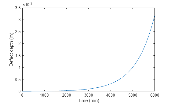
데이터의 여러 세그먼트에서 결함 깊이가 변하는 방식을 플로팅합니다.

plot(expTime,defectDepthVec);
xlabel('Time (min)');
ylabel('Defect depth (m)');

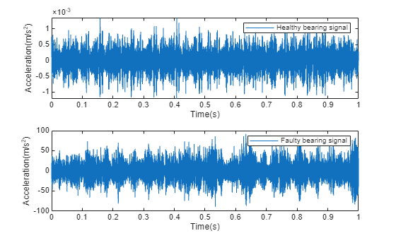
정상 데이터와 결함 데이터를 플로팅합니다.

time = linspace(0,1,fs)';

% healthy bearing signal
subplot(2,1,1);
plot(time,data{1});
xlabel('Time(s)');
ylabel('Acceleration(m/s^2)');
legend('Healthy bearing signal');

% faulty bearing signal
subplot(2,1,2);
plot(time,data{end});
xlabel('Time(s)');
ylabel('Acceleration(m/s^2)');
legend('Faulty bearing signal');

특징 추출

이 섹션에서는 데이터의 각 세그먼트에서 대표적인 특징을 추출합니다. 이러한 특징은 건전성 모니터링 및 예지진단을 위해 사용됩니다. 베어링 진단 및 예지진단을 위한 일반적인 특징에는 시간 영역 특징(RMS, 피크 값, 신호 첨도 등) 또는 주파수 영역 특징(피크 주파수, 평균 주파수 등)이 있습니다.

어느 특징을 사용할지 선택하기 전에 진동 신호 스펙트로그램을 플로팅합니다. 신호를 시간 영역, 주파수 영역 또는 시간-주파수 영역에서 플로팅하면 성능 저하나 고장을 나타내는 신호 패턴을 찾아내는 데 도움이 됩니다.

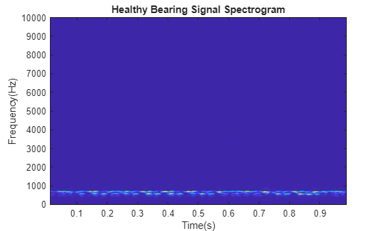
먼저 정상 베어링 데이터의 스펙트로그램을 계산합니다. 500개 데이터 점만큼의 윈도우 크기와 90%의 중첩비(450개 데이터 점에 해당)를 사용합니다. FFT의 점 개수가 512가 되도록 설정합니다. fs는 이전에 정의된 샘플링 주파수를 나타냅니다.

[~,fvec,tvec,P0] = spectrogram(data{1},500,450,512,fs);

P0는 스펙트로그램이고, fvec는 주파수 벡터이고, tvec는 시간 벡터입니다.

정상 베어링 신호의 스펙트로그램을 플로팅합니다.

clf;
imagesc(tvec,fvec,P0)
xlabel('Time(s)');
ylabel('Frequency(Hz)');
title('Healthy Bearing Signal Spectrogram');
axis xy

이번에는 결함 패턴이 발생한 진동 신호의 스펙트로그램을 플로팅합니다. 신호 에너지가 고주파수에 집중된 것을 볼 수 있습니다.

[~,fvec,tvec,Pfinal] = spectrogram(data{end},500,450,512,fs);
imagesc(tvec,fvec,Pfinal)
xlabel('Time(s)');
ylabel('Frequency(Hz)');
title('Faulty Bearing Signal Spectrogram');
axis xy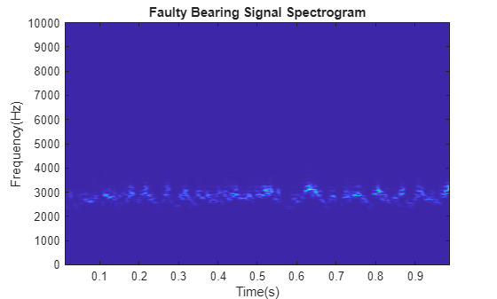

정상 베어링과 결함 베어링의 데이터에 대한 스펙트로그램이 서로 다르므로 스펙트로그램에서 대표적인 특징을 추출하여 상태 모니터링 및 예지진단을 위해 사용할 수 있습니다. 이 예제에서는 스펙트로그램에서 평균 피크 주파수를 건전성 지표로 추출합니다. 스펙트로그램을 $P (t, ω)$ 로 표기합니다. 각 순간 시점에서의 피크 주파수는 다음과 같이 정의됩니다.

$P e a k F r e q (t) = a r g m a x_{ω} P (t, ω)$

평균 피크 주파수는 위에서 정의한 피크 주파수의 평균입니다.

$m e a n P e a k F r e q = \frac{1}{T} \int_{0}^{T} P e a k F r e q (t) d t$

정상 볼 베어링 신호의 평균 피크 주파수를 계산합니다.

[~,I0] = max(P0);               % Find out where the peak frequencies are located.
meanPeakFreq0 = mean(fvec(I0))  % Calculate mean peak frequency.

meanPeakFreq0 = 666.4602

정상 베어링 진동 신호의 평균 피크 주파수는 약 650Hz입니다. 이번에는 결함 베어링 신호의 평균 피크 주파수를 계산합니다. 평균 피크 주파수를 2500Hz 이상으로 이동합니다.

[~,Ifinal] = max(Pfinal);
meanPeakFreqFinal = mean(fvec(Ifinal))

meanPeakFreqFinal = 2.8068e+03

결함 깊이가 그렇게 크지는 않지만 진동 신호에 영향을 주기 시작하는 중간 단계에서 데이터를 검토합니다.

[~,fvec,tvec,Pmiddle] = spectrogram(data{end/2},500,450,512,fs);
imagesc(tvec,fvec,Pmiddle)
xlabel('Time(s)');
ylabel('Frequency(Hz)');
title('Bearing Signal Spectrogram');
axis xy

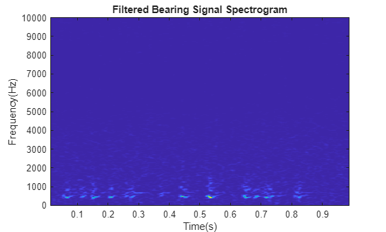
고주파수 잡음 성분이 스펙트로그램 전체에 퍼져 있습니다. 이러한 현상은 원래 진동과 작은 결함으로 인해 발생한 진동의 혼합 효과입니다. 평균 피크 주파수를 정확하게 계산하려면 데이터를 필터링하여 이 고주파수 성분을 제거해야 합니다.

진동 신호에 중앙값 필터를 적용하여 고주파수 잡음 성분을 제거하면서도 고주파수에 있는 유용한 정보를 보존합니다.

dataMiddleFilt = medfilt1(data{end/2},3);

중앙값 필터링을 수행한 후의 스펙트로그램을 플로팅합니다. 고주파수 성분이 표시되지 않습니다.

[~,fvec,tvec,Pmiddle] = spectrogram(dataMiddleFilt,500,450,512,fs);
imagesc(tvec,fvec,Pmiddle)
xlabel('Time(s)');
ylabel('Frequency(Hz)');
title('Filtered Bearing Signal Spectrogram');
axis xy

평균 피크 주파수가 정상 볼 베어링과 결함 볼 베어링을 성공적으로 구분하므로 데이터의 각 세그먼트에서 평균 피크 주파수를 추출합니다.

% Define a progress bar.
h = waitbar(0,'Start to extract features');
% Initialize a vector to store the extracted mean peak frequencies.
meanPeakFreq = zeros(numSamples,1);
for k = 1:numSamples
    % Get most up-to-date data.
    curData = data{k};
    % Apply median filter.
    curDataFilt = medfilt1(curData,3);
    % Calculate spectrogram.
    [~,fvec,tvec,P_k] = spectrogram(curDataFilt,500,450,512,fs);
    % Calculate peak frequency at each time instance.
    [~,I] = max(P_k);
    meanPeakFreq(k) = mean(fvec(I));
    % Show progress bar indicating how many samples have been processed.
    waitbar(k/numSamples,h,'Extracting features');
end
close(h);

추출한 평균 피크 주파수를 시간에 대해 플로팅합니다.

plot(expTime,meanPeakFreq);
xlabel('Time(min)');
ylabel('Mean peak frequency (Hz)');
grid on;

상태 모니터링 및 예지진단

이 섹션에서는 미리 정의된 임계값과 동적 모델을 사용하여 상태 모니터링 및 예지진단을 수행합니다. 상태 모니터링을 위해, 평균 피크 주파수가 미리 정의된 임계값을 초과하면 트리거되는 경보를 만듭니다. 예지진단을 위해, 앞으로 몇 시간 후의 평균 피크 주파수 값을 예측할 동적 모델을 식별합니다. 예측 평균 피크 주파수가 미리 정의된 임계값을 초과하면 트리거되는 경보를 만듭니다.

예측을 사용하면 잠재적인 결함에 더 효과적으로 대비할 수 있고 고장이 발생하기 전에 기계를 중지할 수도 있습니다. 평균 피크 주파수를 시계열로 간주합니다. 평균 피크 주파수의 시계열 모델을 추정하고 이 모델을 사용하여 미래의 값을 전망할 수 있습니다. 처음 200개의 평균 피크 주파수 값을 사용하여 초기 시계열 모델을 만들고, 10개의 새로운 값이 생성되면 마지막 100개의 값을 사용하여 시계열 모델을 업데이트합니다. 이렇게 시계열 모델을 배치 모드로 업데이트하면 순시 추세가 캡처됩니다. 업데이트된 시계열 모델은 앞으로의 10개의 스텝을 미리 계산하여 전망하는 데 사용됩니다.

tStart = 200;               % Start Time
timeSeg = 100;              % Length of data for building dynamic model
forecastLen = 10;           % Define forecast time horizon
batchSize = 10;             % Define batch size for updating the dynamic model

예지진단 및 상태 모니터링을 위해서는 기계를 중지할 시점을 결정하는 임계값을 설정해야 합니다. 이 예제에서는 시뮬레이션에서 생성된 정상 베어링과 결함 베어링의 통계 데이터를 사용하여 임계값을 결정합니다. pdmBearingConditionMonitoringStatistics.mat는 정상 베어링과 결함 베어링의 평균 피크 주파수의 확률 분포를 저장합니다. 확률 분포는 정상 베어링과 결함 베어링의 결함 깊이를 섭동하여 계산됩니다.

url = 'https://www.mathworks.com/supportfiles/predmaint/condition-monitoring-and-prognostics-using-vibration-signals/pdmBearingConditionMonitoringStatistics.mat';
websave('pdmBearingConditionMonitoringStatistics.mat',url);
load pdmBearingConditionMonitoringStatistics.mat

정상 베어링과 결함 베어링의 평균 피크 주파수의 확률 분포를 플로팅합니다.

plot(pFreq,pNormal,'g--',pFreq,pFaulty,'r');
xlabel('Mean peak frequency(Hz)');
ylabel('Probability Distribution');
legend('Normal Bearing','Faulty Bearing');

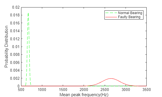
이 플롯을 기반으로, 정상 베어링과 결함 베어링을 구분하고 베어링의 사용을 극대화하기 위해 평균 피크 주파수의 임계값을 2000Hz로 설정합니다.

threshold = 2000;

샘플링 시간을 계산하고 단위를 초로 변환합니다.

samplingTime = 60*(expTime(2)-expTime(1));                  % unit: seconds
tsFeature = iddata(meanPeakFreq(1:tStart),[],samplingTime);

처음 200개의 평균 피크 주파수 데이터를 플로팅합니다.

plot(tsFeature.y)

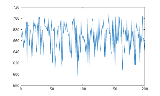
플롯은 초기 데이터가 일정한 레벨과 잡음의 조합임을 보여줍니다. 베어링은 초기에 정상이고 평균 피크 주파수는 유의미하게 변할 것으로 예상되지 않으므로 이는 예상된 동작입니다.

처음 200개의 데이터 점을 사용하여 2차 상태공간 모델을 식별합니다. 모델을 표준형으로 가져오고 샘플링 시간을 지정합니다.

past_sys = ssest(tsFeature,2,'Ts',samplingTime,'Form','canonical')

past_sys =
  Discrete-time identified state-space model:
    x(t+Ts) = A x(t) + K e(t)
       y(t) = C x(t) + e(t)
 
  A = 
            x1       x2
   x1        0        1
   x2   0.9605  0.03942
 
  C = 
       x1  x2
   y1   1   0
 
  K = 
              y1
   x1  -0.003899
   x2   0.003656
 
Sample time: 600 seconds
  
Parameterization:
   CANONICAL form with indices: 2.
   Disturbance component: estimate
   Number of free coefficients: 4
   Use "idssdata", "getpvec", "getcov" for parameters and their uncertainties.

Status:                                               
Estimated using SSEST on time domain data "tsFeature".
Fit to estimation data: 0.2763% (prediction focus)    
FPE: 640, MSE: 602.7

추정된 초기 동적 모델은 피팅 적합도가 낮습니다. 피팅 적합도 메트릭은 NRMSE(정규화된 RMS 오차)로, 다음과 같이 계산됩니다.

$N R M S E = 1 - \frac{‖ x_{t r u e} - x_{p r e d} ‖}{‖ x_{t r u e} - m e a n (x_{t r u e}) ‖}$

여기서 $x_{t r u e}$ 는 실제 값이고 $x_{p r e d}$ 는 예측된 값입니다.

추정 데이터가 일정한 레벨과 잡음의 조합인 경우 $x_{p r e d} \approx m e a n (x_{t r u e})$ 이고 NRMSE는 0에 가깝습니다. 모델을 검증하기 위해 잔차의 자기상관을 플로팅합니다.

resid(tsFeature,past_sys)

플롯에서 볼 수 있듯이 잔차에 상관관계가 없으며 생성된 모델은 유효합니다.

식별된 모델 past_sys를 사용하여 평균 피크 주파수 값을 예측하고 예측된 값의 표준편차를 계산합니다.

[yF,~,~,yFSD] = forecast(past_sys,tsFeature,forecastLen);

예측된 값과 신뢰구간을 플로팅합니다.

tHistory = expTime(1:tStart);
forecastTimeIdx = (tStart+1):(tStart+forecastLen);
tForecast = expTime(forecastTimeIdx);

% Plot historical data, forecast value and 95% confidence interval.
plot(tHistory,meanPeakFreq(1:tStart),'b',...
     tForecast,yF.OutputData,'kx',...
     [tHistory; tForecast], threshold*ones(1,length(tHistory)+forecastLen), 'r--',...
     tForecast,yF.OutputData+1.96*yFSD,'g--',...
     tForecast,yF.OutputData-1.96*yFSD,'g--');

ylim([400, 1.1*threshold]);
ylabel('Mean peak frequency (Hz)');
xlabel('Time (min)');
legend({'Past Data', 'Forecast', 'Failure Threshold', '95% C.I'},...
    'Location','northoutside','Orientation','horizontal');
grid on;

플롯은 평균 피크 주파수의 예측된 값이 임계값보다 훨씬 아래에 있음을 보여줍니다.

이번에는 새로운 데이터가 생겨남에 따라 모델 파라미터를 업데이트하고 예측된 값을 다시 추정합니다. 신호나 예측된 값이 고장 임계값을 초과하는지 검사하는 경보도 만듭니다.

for tCur = tStart:batchSize:numSamples
    %  latest features into iddata object.
    tsFeature = iddata(meanPeakFreq((tCur-timeSeg+1):tCur),[],samplingTime);
    
    % Update system parameters when new data comes in. Use previous model
    % parameters as initial guesses.
    sys = ssest(tsFeature,past_sys);
    past_sys = sys;
    
    % Forecast the output of the updated state-space model. Also compute
    % the standard deviation of the forecasted output.
    [yF,~,~,yFSD]  = forecast(sys, tsFeature, forecastLen);
    
    % Find the time corresponding to historical data and forecasted values.
    tHistory = expTime(1:tCur);
    forecastTimeIdx = (tCur+1):(tCur+forecastLen);
    tForecast = expTime(forecastTimeIdx);
    
    % Plot historical data, forecasted mean peak frequency value and 95%
    % confidence interval.
    plot(tHistory,meanPeakFreq(1:tCur),'b',...
              tForecast,yF.OutputData,'kx',...
              [tHistory; tForecast], threshold*ones(1,length(tHistory)+forecastLen), 'r--',...
              tForecast,yF.OutputData+1.96*yFSD,'g--',...
              tForecast,yF.OutputData-1.96*yFSD,'g--');

    ylim([400, 1.1*threshold]);
    ylabel('Mean peak frequency (Hz)');
    xlabel('Time (min)');
    legend({'Past Data', 'Forecast', 'Failure Threshold', '95% C.I'},...
           'Location','northoutside','Orientation','horizontal');
    grid on;
    
    % Display an alarm when actual monitored variables or forecasted values exceed
    % failure threshold.
    if(any(meanPeakFreq(tCur-batchSize+1:tCur)>threshold))
        disp('Monitored variable exceeds failure threshold');
        break;
    elseif(any(yF.y>threshold))
        % Estimate the time when the system will reach failure threshold.
        tAlarm = tForecast(find(yF.y>threshold,1));
        disp(['Estimated to hit failure threshold in ' num2str(tAlarm-tHistory(end)) ' minutes from now.']);
        break;
    end
end

Estimated to hit failure threshold in 80 minutes from now.

가장 최근의 시계열 모델을 검토합니다.

sys

sys =
  Discrete-time identified state-space model:
    x(t+Ts) = A x(t) + K e(t)
       y(t) = C x(t) + e(t)
 
  A = 
           x1      x2
   x1       0       1
   x2  0.2624   0.746
 
  C = 
       x1  x2
   y1   1   0
 
  K = 
           y1
   x1  0.3902
   x2  0.3002
 
Sample time: 600 seconds
  
Parameterization:
   CANONICAL form with indices: 2.
   Disturbance component: estimate
   Number of free coefficients: 4
   Use "idssdata", "getpvec", "getcov" for parameters and their uncertainties.

Status:                                               
Estimated using SSEST on time domain data "tsFeature".
Fit to estimation data: 92.53% (prediction focus)     
FPE: 499.3, MSE: 442.7

피팅 적합도가 90% 이상으로 증가하고 추세가 올바르게 캡처됩니다.

결론

이 예제에서는 측정된 데이터로부터 특징을 추출하여 상태 모니터링 및 예지진단을 수행하는 방법을 보여주었습니다. 추출된 특징을 기반으로 동적 모델이 생성 및 검증되었고 실제 고장이 발생하기 전에 조치를 취할 수 있도록 고장 수명을 예측하는 데 사용되었습니다.

진동 신호를 사용한 상태 모니터링 및 예지진단

데이터 설명

특징 추출

상태 모니터링 및 예지진단

결론

관련 항목