Magnetic Flux Density in Electromagnet

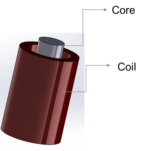
This example shows how to solve a 3-D magnetostatic problem for a solenoid with a finite length iron core. Using a ferromagnetic core with high permeability, such as an iron core, inside a solenoid increases magnetic field and flux density. In this example, you find the magnetic flux density for a geometry consisting of a coil with a finite length core in a cylindrical air domain.

The first part of the example solves the magnetostatic problem using a 3-D model. The second part solves the same problem using an axisymmetric 2-D model to speed up computations.

3-D Model of Coil with Core

Create geometries consisting of three cylinders: a solid circular cylinder models the core, an annular circular cylinder models the coil, and a larger circular cylinder models the air around the coil.

coreGm = multicylinder(0.03,0.1);
coilGm = multicylinder([0.05 0.07],0.2,Void=[1 0]);
airGm = multicylinder(1,2);

Position the core and coil so that the finite length core is located near the top of coil.

coreGm = translate(coreGm,[0 0 1.025]);
coilGm = translate(coilGm,[0 0 0.9]);

Combine the geometries and plot the result.

gm = addCell(airGm,coreGm);
gm = addCell(gm,coilGm);
pdegplot(gm,FaceAlpha=0.2,CellLabels="on")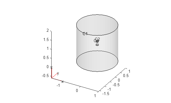

Zoom in to see the cell labels on the core and coil.

figure
pdegplot(gm,FaceAlpha=0.2,CellLabels="on")
axis([-0.1 0.1 -0.1 0.1 0.8 1.2])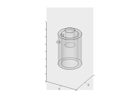

Create an femodel object for magnetostatic analysis and assign air geometry to the model.

model = femodel(AnalysisType="magnetostatic", ...
                Geometry=gm);

Specify the vacuum permeability value in the SI system of units.

model.VacuumPermeability = 1.2566370614E-6;

Specify a relative permeability of 1 for all domains.

model.MaterialProperties = ...
    materialProperties(RelativePermeability=1);

Now specify the large relative permeability of the core.

model.MaterialProperties(2) = ...
    materialProperties(RelativePermeability=10000);

Create a function that defines counterclockwise current density in the coil.

function f3D = windingCurrent3D(region,~)
[TH,~,~] = cart2pol(region.x,region.y,region.z);
f3D = -5E6*[sin(TH); -cos(TH); zeros(size(TH))];
end

Assign an excitation current using this function.

model.CellLoad(3) = ...
    cellLoad(CurrentDensity=@windingCurrent3D);

Assign the zero magnetic potential on the outer surface of the air domain. First, plot the geometry with face labels.

pdegplot(model.Geometry,FaceAlpha=0.5, ...
                        FaceLabels="on")

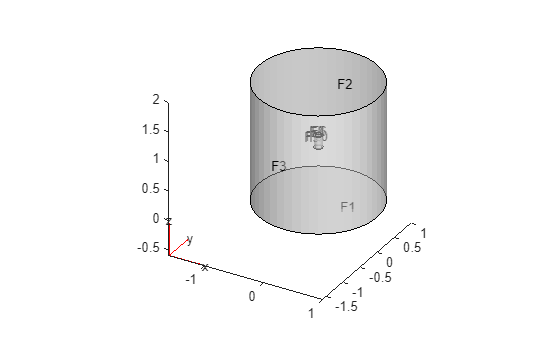
Specify that the magnetic potential on faces forming the outer surface of the air domain is 0.

model.FaceBC(1:3) = faceBC(MagneticPotential=[0;0;0]);

Generate a mesh where only the core and coil regions are well refined and the air domain is relatively coarse to limit the size of the problem.

internalFaces = cellFaces(model.Geometry,2:3);
model = generateMesh(model,Hface={internalFaces,0.007});

Solve the model.

R = solve(model)

R = 
  MagnetostaticResults with properties:

      MagneticPotential: [1×1 FEStruct]
          MagneticField: [1×1 FEStruct]
    MagneticFluxDensity: [1×1 FEStruct]
                   Mesh: [1×1 FEMesh]

Find the magnitude of the flux density.

Bmag = sqrt(R.MagneticFluxDensity.Bx.^2 + ...
            R.MagneticFluxDensity.By.^2 + ...
            R.MagneticFluxDensity.Bz.^2);

Find the mesh elements belonging to the core and the coil.

coreAndCoilElem = findElements(R.Mesh, ...
                               "region", ...
                               Cell=[2 3]);

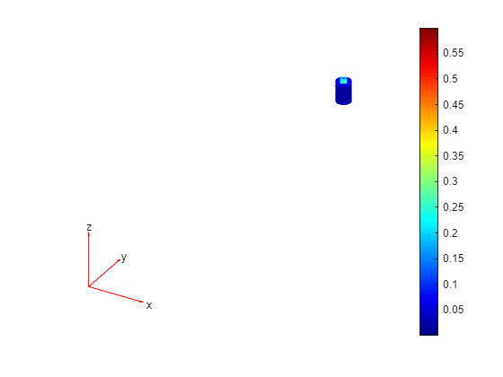
Plot the magnitude of the flux density on the core and coil.

pdeplot3D(R.Mesh.Nodes, ...
          R.Mesh.Elements(:,coreAndCoilElem), ...
          ColorMapData=Bmag)

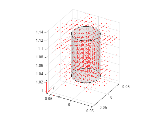
Interpolate the flux to a grid covering the portion of the geometry near the core.

x = -0.05:0.01:0.05;
z = 1.02:0.01:1.14;
y = x;
[X,Y,Z] = meshgrid(x,y,z);
intrpBcore = R.interpolateMagneticFlux(X,Y,Z); 

Reshape intrpBcore.Bx, intrpBcore.By, and intrpBcore.Bz and plot the magnetic flux density as a vector plot.

Bx = reshape(intrpBcore.Bx,size(X));
By = reshape(intrpBcore.By,size(Y));
Bz = reshape(intrpBcore.Bz,size(Z));

quiver3(X,Y,Z,Bx,By,Bz,Color="r")
hold on
pdegplot(coreGm,FaceAlpha=0.2);

2-D Axisymmetric Model of Coil with Core

Now, simplify this 3-D problem to 2-D using the symmetry around the axis of rotation.

First, create the geometry. The axisymmetric section consists of two small rectangular regions (the core and coil) located within a large rectangular region (air).

R1 = [3,4,0.0,1,1,0.0,0,0,2,2]';
R2 = [3,4,0,0.03,0.03,0,1.025,1.025,1.125,1.125]';
R3 = [3,4,0.05,0.07,0.07,0.05,0.90,0.90,1.10,1.10]';
ns = char('R1','R2','R3');
sf = 'R1+R2+R3';
gdm = [R1, R2, R3];
g = decsg(gdm,sf,ns');

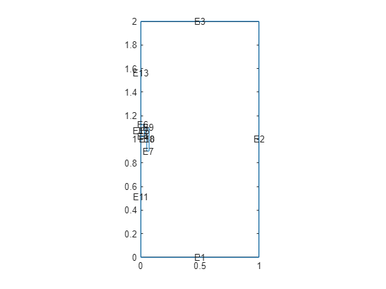
Plot the geometry with the face labels.

pdegplot(g,FaceLabels="on")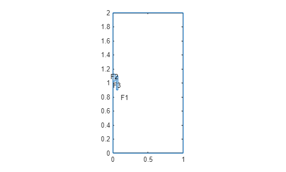

Zoom in to see the face labels on the core and coil.

figure
pdegplot(g,FaceLabels="on")
axis([0 0.1 0.8 1.2])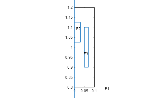

Create an femodel object for magnetostatic axisymmetric analysis and include the geometry.

model = femodel(AnalysisType="magnetostatic", ...
                Geometry=g);
model.PlanarType = "axisymmetric";

Specify the vacuum permeability value in the SI system of units.

model.VacuumPermeability = 1.2566370614E-6;

Specify a relative permeability of 1 for all domains.

model.MaterialProperties = ...
    materialProperties(RelativePermeability=1);

Now specify the large relative permeability of the core.

model.MaterialProperties(3) = ...
    materialProperties(RelativePermeability=10000);

Specify the current density in the coil. For an axisymmetric model, use the constant current value.

model.FaceLoad(2) = ...
    faceLoad(CurrentDensity=5E6);

Assign zero magnetic potential on the outer edges of the air domain as the boundary condition. First, plot the geometry with edge labels.

pdegplot(model.Geometry,FaceAlpha=0.2, ...
                        EdgeLabels="on")

Specify that the magnetic potential on the outer edges of the air domain is 0.

model.EdgeBC([2 8]) = edgeBC(MagneticPotential=0);

Generate a mesh where only the core and coil regions are well refined and the air domain is relatively coarse to limit the size of the problem.

internalEdges = faceEdges(model.Geometry,2:3);
model = generateMesh(model,Hedge={internalEdges,0.007});

Solve the model.

R = solve(model);

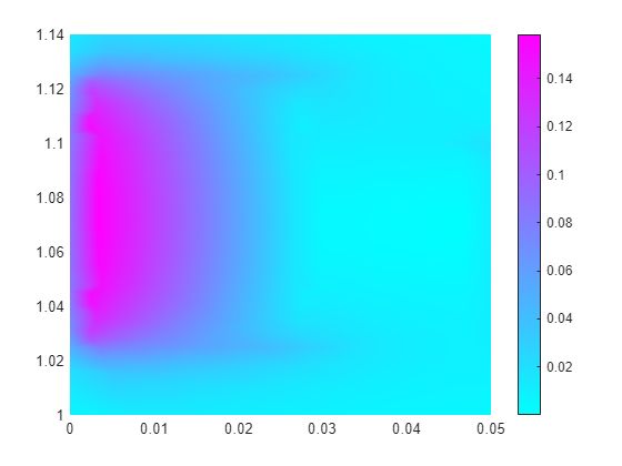
Find the magnitude of the flux density.

Bmag = sqrt(R.MagneticFluxDensity.Bx.^2 + ...
            R.MagneticFluxDensity.By.^2);

Plot the magnitude of the flux density on the core and coil.

pdeplot(R.Mesh,XYData=Bmag)
xlim([0,0.05]);
ylim([1.0,1.14])

Interpolate the flux to a grid covering the portion of the geometry near the core.

x = 0:0.01:0.05;
y = 1.02:0.01:1.14;
[X,Y] = meshgrid(x,y);
intrpBcore = R.interpolateMagneticFlux(X,Y);

Reshape intrpBcore.Bx and intrpBcore.By and plot the magnetic flux density as a vector plot.

Bx = reshape(intrpBcore.Bx,size(X));
By = reshape(intrpBcore.By,size(Y));

quiver(X,Y,Bx,By,Color="r")
hold on
pdegplot(model.Geometry);
xlim([0,0.07]);
ylim([1.0,1.14])

References

[1] Thierry Lubin, Kévin Berger, Abderrezak Rezzoug. "Inductance and Force Calculation for Axisymmetric Coil Systems Including an Iron Core of Finite Length." Progress In Electromagnetics Research B, EMW Publishing 41 (2012): 377-396. https://hal.science/hal-00711310.