Magnetic Field in Two-Pole Electric Motor

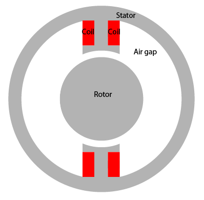
Find the static magnetic field induced by the stator windings in a two-pole electric motor. Assuming that the motor is long and the end effects are negligible, you can use a 2-D model. The geometry consists of three regions:

• Two ferromagnetic pieces: the stator and the rotor, made of transformer steel

• The air gap between the stator and the rotor

• The armature copper coil carrying the DC current

The magnetic permeability of air and of copper are both close to the magnetic permeability of a vacuum, μ = μ₀. The magnetic permeability of the stator and the rotor is μ = 5000μ₀. The current density J is 0 everywhere except in the coil, where it is 10 A/m².

The geometry of the problem makes the magnetic vector potential A symmetric with respect to the y-axis and antisymmetric with respect to the x-axis. Therefore, you can limit the domain to x ≥ 0, y ≥ 0, with the default boundary condition

$$n\cdot \left(\frac{1}{\mu }\nabla A\right)=0$$

on the x-axis and the boundary condition A = 0 on the y-axis. Because the field outside the motor is negligible, you can use the boundary condition A = 0 on the exterior boundary.

First, create the geometry in the PDE Modeler app. The geometry of this electric motor is a union of five circles and two rectangles. To draw the geometry, enter the following commands in the MATLAB^® Command Window:

pdecirc(0,0,1,'C1') 
pdecirc(0,0,0.8,'C2') 
pdecirc(0,0,0.6,'C3')
pdecirc(0,0,0.5,'C4') 
pdecirc(0,0,0.4,'C5') 
pderect([-0.2 0.2 0.2 0.9],'R1') 
pderect([-0.1 0.1 0.2 0.9],'R2') 
pderect([0 1 0 1],'SQ1')

Reduce the geometry to the first quadrant by intersecting it with a square. To do this, enter (C1+C2+C3+C4+C5+R1+R2)*SQ1 in the Set formula field.

From the PDE Modeler app, export the geometry description matrix, set formula, and name-space matrix to the MATLAB workspace by selecting Export Geometry Description, Set Formula, Labels... from the Draw menu.

In the MATLAB Command Window, use the decsg function to decompose the exported geometry into minimal regions. This command creates an AnalyticGeometry object d1. Plot the geometry d1.

[d1,bt1] = decsg(gd,sf,ns);
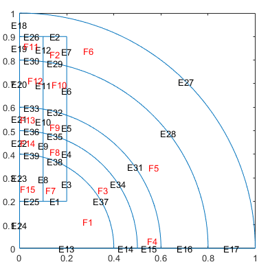
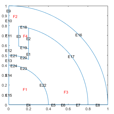
pdegplot(d1,EdgeLabels="on",FaceLabels="on")

Remove unnecessary edges using the csgdel function. Specify the edges to delete as a vector of edge IDs. Plot the resulting geometry.

[d2,bt2] = csgdel(d1,bt1,[1 3 8 25 7 2 12 26 30 33 4 9 34 10 31]);
pdegplot(d2,EdgeLabels="on",FaceLabels="on")

Create an femodel object for magnetostatic analysis and include the geometry in the model.

model = femodel(AnalysisType="magnetostatic", ...
                Geometry=d2);

Specify the vacuum permeability value in the SI system of units.

model.VacuumPermeability = 1.2566370614E-6;

Specify the relative permeability of the air gap and copper coil, which correspond to the faces 3 and 4 of the geometry.

model.MaterialProperties([3 4]) = ...
    materialProperties(RelativePermeability=1);

Specify the relative permeability of the stator and the rotor, which correspond to the faces 1 and 2 of the geometry.

model.MaterialProperties([1 2]) = ...
    materialProperties(RelativePermeability=5000);

Specify the current density in the coil.

model.FaceLoad(4) = faceLoad(CurrentDensity=10);

Apply the zero magnetic potential condition to all boundaries, except the edges along the x-axis. The edges along the x-axis retain the default boundary condition.

model.EdgeBC([16 9 10 11 12 13 14 15]) = ...
    edgeBC(MagneticPotential=0);

Generate the mesh.

model = generateMesh(model);

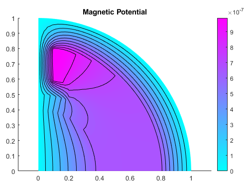
Solve the model and plot the magnetic potential. Use the Contour parameter to display equipotential lines.

R = solve(model);
figure
pdeplot(R.Mesh, ...
        XYData=R.MagneticPotential, ...
        Contour="on")
title("Magnetic Potential")

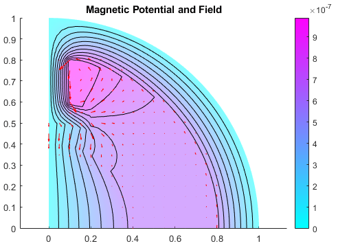
Add the magnetic field data to the plot. Use the FaceAlpha parameter to make the quiver plot for magnetic field more visible.

figure
pdeplot(R.Mesh,XYData=R.MagneticPotential, ...
               FlowData=[R.MagneticField.Hx, ...
                         R.MagneticField.Hy], ...
               Contour="on", ...
               FaceAlpha=0.5)
title("Magnetic Potential and Field")