캐비티가 있는 블록의 열 전달

이 예제에서는 캐비티(cavity)가 있는 블록의 열 분포를 구하는 방법을 보여줍니다.

사각형 모양의 균열 또는 캐비티가 있는 블록을 생각해 보겠습니다. 블록의 왼쪽 면은 섭씨 100도로 가열됩니다. 블록의 오른쪽 면에서는 열이 블록에서 주변 공기로 $-10\mathit{W}/{\mathit{m}}^2$의 일정한 속도로 흐릅니다. 다른 모든 경계는 절연되어 있습니다. 시작 시간 ${\mathit{t}}_0=0$에서 블록의 온도는 0도입니다. 목표는 처음 5초 동안의 열 분포를 모델링하는 것입니다.

지오메트리를 사용하여 모델 만들기

이 열 전달 문제를 푸는 첫 번째 단계는 캐비티가 있는 블록을 나타내는 지오메트리를 사용하여 열 해석을 위한 femodel 객체를 만드는 것입니다.

model = femodel(AnalysisType="thermalTransient", ...
                Geometry=@crackg);

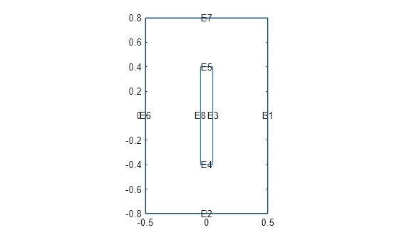
지오메트리 플로팅하기

모서리 레이블을 포함하여 지오메트리를 플로팅합니다.

pdegplot(model,EdgeLabels="on");
axis equal

물질의 열 속성 지정하기

물질의 열전도도, 질량 밀도, 비열을 지정합니다.

model.MaterialProperties = ...
            materialProperties(ThermalConductivity=1, ...
                               MassDensity=1, ...
                               SpecificHeat=1);

경계 조건 적용하기

왼쪽 모서리의 온도를 100으로 지정하고 오른쪽 모서리를 통한 외부로의 일정한 열 유량을 -10으로 지정합니다. 툴박스는 다른 모든 경계에 대해 디폴트 절연 경계 조건을 사용합니다.

model.EdgeBC(6) = edgeBC(Temperature=100);
model.EdgeLoad(1) = edgeLoad(Heat=-10);

초기 조건 설정하기

온도의 초기값을 0으로 설정합니다.

model.FaceIC = faceIC(Temperature=0);

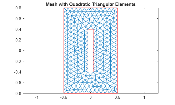
메시 생성하기

메시를 생성하고 결과를 모델에 할당합니다. 이 할당을 수행하면 모델의 Geometry 속성에 저장된 메시가 업데이트됩니다. 메시를 플로팅합니다.

model = generateMesh(model);

figure
pdemesh(model);
title("Mesh with Quadratic Triangular Elements")
axis equal

풀이 시간 지정하기

풀이 시간을 0초부터 5초까지 1/2초 간격으로 설정합니다.

tlist = 0:0.5:5;

해 계산하기

solve 함수를 사용하여 해를 계산합니다.

results = solve(model,tlist)

results = 
  TransientThermalResults with properties:

      Temperature: [1308×11 double]
    SolutionTimes: [0 0.5000 1 1.5000 2 2.5000 3 3.5000 4 4.5000 5]
       XGradients: [1308×11 double]
       YGradients: [1308×11 double]
       ZGradients: []
             Mesh: [1×1 FEMesh]

열 플럭스 계산하기

열 플럭스 밀도를 계산합니다.

[qx,qy] = evaluateHeatFlux(results);

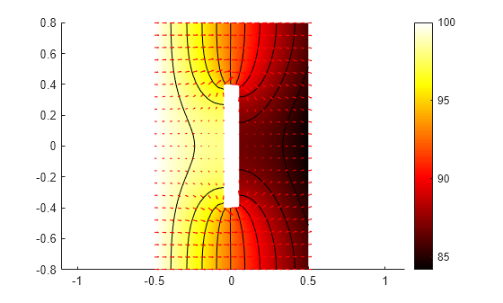
온도 분포 및 열 플럭스 플로팅하기

등고선 플롯을 사용하여 최종 시간 스텝인 t = 5.0초에서 등온선과 함께 해를 플로팅하고, 화살표를 사용하여 열 플럭스 벡터장을 플로팅합니다.

figure
pdeplot(results.Mesh,XYData=results.Temperature(:,end), ...
                     Contour="on",...
                     FlowData=[qx(:,end),qy(:,end)], ...
                     ColorMap="hot")
axis equal