Specify Nonconstant Boundary Conditions

When solving PDEs with nonconstant boundary conditions, specify these conditions by using function handles. This example shows how to write functions to represent nonconstant boundary conditions for PDE problems.

Geometry and Mesh

Create a model.

model = createpde;

Include a unit square geometry in the model and plot the geometry.

geometryFromEdges(model,@squareg);
pdegplot(model,"EdgeLabels","on")
xlim([-1.1 1.1])
ylim([-1.1 1.1])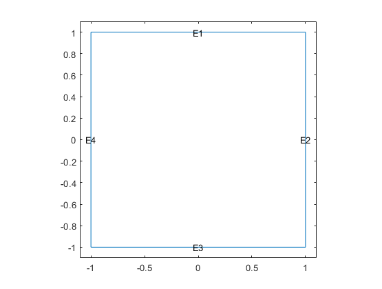

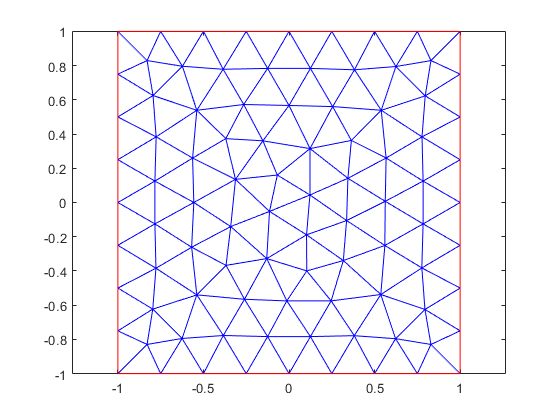
Generate a mesh with a maximum edge length of 0.25. Plot the mesh.

generateMesh(model,"Hmax",0.25);
figure
pdemesh(model)

Scalar PDE Problem with Nonconstant Boundary Conditions

Write functions to represent the nonconstant boundary conditions on edges 1 and 3. Each function must accept two input arguments, location and state. The solvers automatically compute and populate the data in the location and state structure arrays and pass this data to your function.

Write a function that returns the value $$u\left(x,y\right)=52+20x$$ to represent the Dirichlet boundary condition for edge 1.

function bc = bcfuncD(location,state)
    bc = 52 + 20*location.x;
    scatter(location.x,location.y,"filled","black");
    hold on
end

Write a function that returns the value $$u\left(x,y\right)=\cos \left(x^2\right)$$ to represent the Neumann boundary condition for edge 3.

function bc = bcfuncN(location,state)
    bc = cos(location.x).^2;
    scatter(location.x,location.y,"filled","red");
    hold on
end

The scatter plot command in each of these functions enables you to visualize the location data used by the toolbox. For Dirichlet boundary conditions, the location data (black markers on edge 1) corresponds with the mesh nodes. Each element of a quadratic mesh has nodes at its corners and edge centers. For Neumann boundary conditions, the location data (red markers on edge 3) corresponds with the quadrature integration points.

Specify the boundary condition for edges 1 and 3 using the functions that you wrote.

applyBoundaryCondition(model,"dirichlet", ...
                             "Edge",1, ...
                             "u",@bcfuncD);
applyBoundaryCondition(model,"neumann", ...
                             "Edge",3, ...
                             "g",@bcfuncN);

Specify the PDE coefficients.

specifyCoefficients(model,"m",0,"d",0,"c",1, ...
                          "a",0,"f",10);

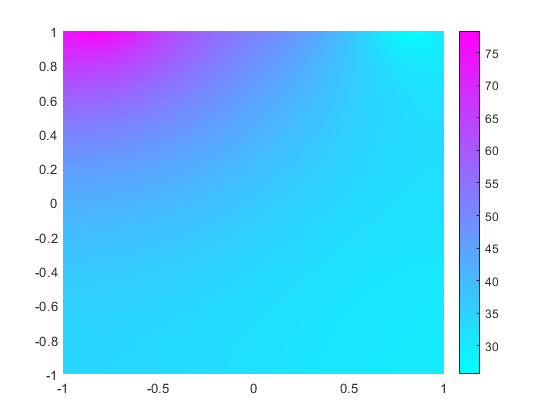
Solve the equation and plot the solution.

results = solvepde(model);

figure
pdeplot(model,"XYData",results.NodalSolution)

Anonymous Functions for Nonconstant Boundary Conditions

If the dependency of a boundary condition on coordinates, time, or solution is simple, you can use an anonymous function to represent the nonconstant boundary condition. Thus, you can implement the linear interpolation shown earlier in this example as the bcfuncD function, as this anonymous function.

bcfuncD = @(location,state)52 + 20*location.x;

Specify the boundary condition for edge 1.

applyBoundaryCondition(model,"dirichlet", ...
                             "Edge",1, ...
                             "u",bcfuncD);

Additional Arguments

If a function that represents a nonconstant boundary condition requires more arguments than location and state, follow these steps:

1. Write a function that takes the location and state arguments and the additional arguments.

2. Wrap that function with an anonymous function that takes only the location and state arguments.

For example, define boundary conditions on edge 1 as $$u\left(x,y\right)=52a^2+20bx+c$$. First, write the function that takes the arguments a, b, and c in addition to the location and state arguments.

function bc = bcfunc_abc(location,state,a,b,c)
    bc = 52*a^2 + 20*b*location.x + c;    
end

Because a function defining nonconstant boundary conditions must have exactly two arguments, wrap the bcfunc_abc function with an anonymous function.

bcfunc_add_args = @(location,state) bcfunc_abc(location,state,1,2,3);

Now you can use bcfunc_add_args to specify a boundary condition for edge 1.

applyBoundaryCondition(model,"dirichlet", ...
                             "Edge",1, ...
                             "u",bcfunc_add_args);

System of PDEs

Create a model for a system of two equations.

model = createpde(2);

Use the same unit square geometry that you used for the scalar PDE problem.

geometryFromEdges(model,@squareg);

The first component on edge 1 satisfies the equation $$u_1\left(x,y\right)=52+20x+10\sin \left(\pi x^3\right)$$. The second component on edge 1 satisfies the equation $$u_1\left(x,y\right)=52-20x-10\sin \left(\pi x^3\right)$$.

Write a function file myufun.m that incorporates these equations.

function bcMatrix = myufun(location,state)
bcMatrix = [52 + 20*location.x + 10*sin(pi*(location.x.^3));
            52 - 20*location.x - 10*sin(pi*(location.x.^3))];
end

Specify the boundary condition for edge 1 using the myufun function.

applyBoundaryCondition(model,"dirichlet","Edge",1, ...
                                         "u",@myufun);

Specify the PDE coefficients.

specifyCoefficients(model,"m",0,"d",0,"c",1, ...
                          "a",0,"f",[10;-10]);

Generate a mesh.

generateMesh(model);

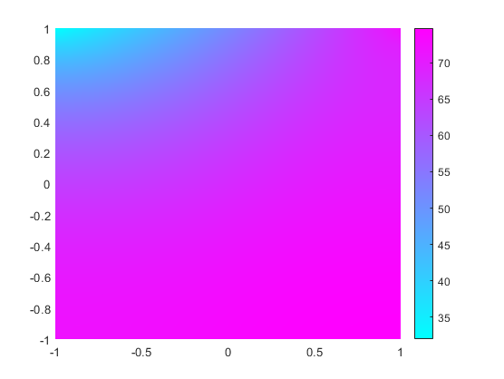
Solve the system and plot the solution.

results = solvepde(model);
u = results.NodalSolution;

figure
pdeplot(model,"XYData",u(:,1))

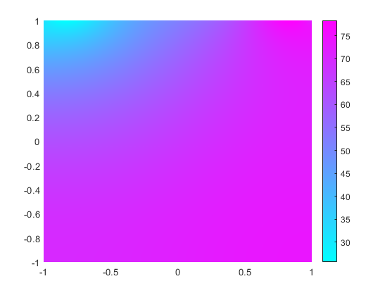
figure
pdeplot(model,"XYData",u(:,2))