이 번역 페이지는 최신 내용을 담고 있지 않습니다. 최신 내용을 영문으로 보려면 여기를 클릭하십시오.

제약 조건이 있는 비선형 최적화 풀기(문제 기반)

이 예제에서는 문제 기반 접근법을 사용하여 비선형 제약 조건을 가진 비선형 목적 함수의 최솟값을 찾는 방법을 보여줍니다. 유사한 문제에 대한 해를 보여주는 비디오는 Problem-Based Nonlinear Programming을 참조하십시오.

문제 기반 접근법을 사용하여 비선형 목적 함수의 최솟값을 구하기 위해 먼저 목적 함수를 파일이나 익명 함수로 작성합니다. 이 예제에서 사용하는 목적 함수는 다음과 같습니다.

$$f(x,y)=e^x(4x^2+2y^2+4xy+2y-1).$$

type objfunx

function f = objfunx(x,y)
f = exp(x).*(4*x.^2 + 2*y.^2 + 4*x.*y + 2*y - 1);
end

최적화 문제 변수 x와 y를 만듭니다.

x = optimvar('x');
y = optimvar('y');

목적 함수를 최적화 변수의 표현식으로 만듭니다.

obj = objfunx(x,y);

obj를 사용하는 최적화 문제를 목적 함수로 만듭니다.

prob = optimproblem('Objective',obj);

다음과 같이 비선형 제약 조건을 지정하여 해가 기울어진 타원에 있도록 합니다.

$$\frac{xy}{2}+(x+2{)}^2+\frac{(y-2{)}^2}{2}\le 2.$$

제약 조건을 최적화 변수의 부등식으로 만듭니다.

TiltEllipse = x.*y/2 + (x+2).^2 + (y-2).^2/2 <= 2;

문제에 제약 조건을 포함시킵니다.

prob.Constraints.constr = TiltEllipse;

초기점을 x = –3, y = 3으로 나타내는 구조체를 만듭니다.

x0.x = -3;
x0.y = 3;

문제를 검토합니다.

show(prob)

  OptimizationProblem : 

	Solve for:
       x, y

	minimize :
       (exp(x) .* (((((4 .* x.^2) + (2 .* y.^2)) + ((4 .* x) .* y)) + (2 .* y)) - 1))


	subject to constr:
       ((((x .* y) ./ 2) + (x + 2).^2) + ((y - 2).^2 ./ 2)) <= 2
     

문제를 풉니다.

[sol,fval] = solve(prob,x0)

Solving problem using fmincon.

Local minimum found that satisfies the constraints.

Optimization completed because the objective function is non-decreasing in 
feasible directions, to within the value of the optimality tolerance,
and constraints are satisfied to within the value of the constraint tolerance.

sol = struct with fields:
    x: -5.2813
    y: 4.6815

fval = 0.3299

다른 시작점을 사용해 봅니다.

x0.x = -1;
x0.y = 1;
[sol2,fval2] = solve(prob,x0)

Solving problem using fmincon.

Feasible point with lower objective function value found.


Local minimum found that satisfies the constraints.

Optimization completed because the objective function is non-decreasing in 
feasible directions, to within the value of the optimality tolerance,
and constraints are satisfied to within the value of the constraint tolerance.

sol2 = struct with fields:
    x: -0.8210
    y: 0.6696

fval2 = 0.7626

타원, 목적 함수 경로 및 두 개의 해를 플로팅합니다.

f = @objfunx;
g = @(x,y) x.*y/2+(x+2).^2+(y-2).^2/2-2;
rnge = [-5.5 -0.25 -0.25 7];
fimplicit(g,'k-')
axis(rnge);
hold on
fcontour(f,rnge,'LevelList',logspace(-1,1))
plot(sol.x,sol.y,'ro','LineWidth',2)
plot(sol2.x,sol2.y,'ko','LineWidth',2)
legend('Constraint','f Contours','Global Solution','Local Solution','Location','northeast');
hold off

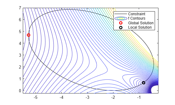
해가 비선형 제약 조건 경계에 있습니다. 등고선 플롯은 이러한 해가 유일한 국소 최솟값임을 보여줍니다. 또한, 플롯은 [–2,3/2] 근처에 정상점이 있고 [–2,0]과 [–1,4] 근처에 국소 최댓값이 있음을 보여줍니다.

fcn2optimexpr을 사용하여 목적 함수 변환하기

일부 목적 함수 또는 소프트웨어 버전의 경우 fcn2optimexpr을 사용하여 비선형 함수를 최적화 표현식으로 변환해야 합니다. Supported Operations for Optimization Variables and Expressions 항목과 Convert Nonlinear Function to Optimization Expression 항목을 참조하십시오. fcn2optimexpr 호출에 변수 x와 y를 전달하여 각 objfunx 입력에 대응하는 최적화 변수를 나타냅니다.

obj = fcn2optimexpr(@objfunx,x,y);

obj를 사용하는 최적화 문제를 전과 같이 목적 함수로 만듭니다.

prob = optimproblem('Objective',obj);

나머지 풀이 과정은 동일합니다.

Copyright 2018–2020 The MathWorks, Inc.

참고 항목

fcn2optimexpr

관련 항목

• 문제 기반 최적화 워크플로
• 문제 기반 비선형 최적화