상미분 방정식(ODE) 피팅하기

R2026b

이 예제에서는 두 가지 방식으로 ODE의 파라미터를 데이터에 피팅하는 방법을 보여줍니다. 첫 번째 방법에서는 초기 파라미터에 민감하게 의존하는 유명한 ODE인 로렌츠 연립방정식의 해 중 일부에 대한 등속 원형 경로의 직관적인 피팅을 보여줍니다. 두 번째 방법에서는 등속 원형 경로를 피팅하기 위해 로렌츠 방정식의 파라미터를 수정하는 방법을 보여줍니다. 응용 사례에 적합한 접근법을 모델로 삼아 미분 방정식을 데이터에 피팅할 수 있습니다.

로렌츠 방정식: 정의 및 수치 해

로렌츠 연립방정식은 연립상미분방정식입니다(로렌츠 방정식 참조). 실수 상수 $$\sigma ,\rho ,\beta$$에 대해 연립방정식은 다음과 같습니다.

$$\begin{array}{l}\frac{dx}{dt}=\sigma (y-x)\\ \frac{dy}{dt}=x(\rho -z)-y\\ \frac{dz}{dt}=xy-\beta z.\end{array}$$

어떤 민감한 연립방정식에 대한 파라미터의 로렌츠 값이 $$\sigma =10,\beta =8/3,\rho =28$$입니다. [x(0),y(0),z(0)] = [10,20,10]에서 시작해 시간 0부터 100까지 연립방정식의 전개를 살펴봅니다.

sigma = 10;
beta = 8/3;
rho = 28;
f = @(t,a) [-sigma*a(1) + sigma*a(2); rho*a(1) - a(2) - a(1)*a(3); -beta*a(3) + a(1)*a(2)];
xt0 = [10,20,10];
[tspan,a] = ode45(f,[0 100],xt0);     % Runge-Kutta 4th/5th order ODE solver
figure
plot3(a(:,1),a(:,2),a(:,3))
view([-10.0 -2.0])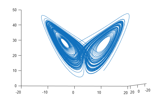

전개 양상이 매우 복잡합니다. 하지만 짧은 시간 간격에서는 균일한 원을 그리는 것처럼 보입니다. 시간 간격 [0,1/10]에 대해 해를 플로팅합니다.

[tspan,a] = ode45(f,[0 1/10],xt0);     % Runge-Kutta 4th/5th order ODE solver
figure
plot3(a(:,1),a(:,2),a(:,3))
view([-30 -70])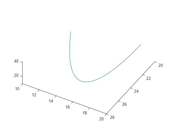

ODE 해에 원형 경로 피팅하기

원형 경로의 방정식에는 다음과 같이 여러 개의 파라미터가 있습니다.

• x-y 평면에서 경로의 각도 $$\theta (1)$$

• x축을 따라 기울어진 평면의 각도 $$\theta (2)$$

• 반지름 R

• 속도 V

• 시간 0으로부터의 이동 t0

• 공간 delta에서의 3차원 이동

이러한 파라미터의 관점에서 시간 xdata에 대한 원형 경로의 위치를 결정하십시오.

function f = fitlorenzfn(x,xdata)

theta = x(1:2);
R = x(3);
V = x(4);
t0 = x(5);
delta = x(6:8);
f = zeros(length(xdata),3);
f(:,3) = R*sin(theta(1))*sin(V*(xdata - t0)) + delta(3);
f(:,1) = R*cos(V*(xdata - t0))*cos(theta(2)) ...
    - R*sin(V*(xdata - t0))*cos(theta(1))*sin(theta(2)) + delta(1);
f(:,2) = R*sin(V*(xdata - t0))*cos(theta(1))*cos(theta(2)) ...
    - R*cos(V*(xdata - t0))*sin(theta(2)) + delta(2);
end

ODE 해에 지정된 시간에 로렌츠 연립방정식에 대한 최적 피팅의 원형 경로를 찾으려면 lsqcurvefit을 사용하십시오. 다양한 파라미터들이 적절한 한계 내에 있도록 파라미터의 범위를 정하십시오.

lb = [-pi/2,-pi,5,-15,-pi,-40,-40,-40];
ub = [pi/2,pi,60,15,pi,40,40,40];
theta0 = [0;0];
R0 = 20;
V0 = 1;
t0 = 0;
delta0 = zeros(3,1);
x0 = [theta0;R0;V0;t0;delta0];
[xbest,resnorm,residual] = lsqcurvefit(@fitlorenzfn,x0,tspan,a,lb,ub);

Local minimum possible.

lsqcurvefit stopped because the final change in the sum of squares relative to 
its initial value is less than the value of the function tolerance.

<stopping criteria details>

ODE 해의 시간에 최적 피팅의 원형 점을 로렌츠 연립방정식의 해와 함께 플로팅합니다.

soln = a + residual;
hold on
plot3(soln(:,1),soln(:,2),soln(:,3),"r")
legend("ODE Solution","Circular Arc")
hold off

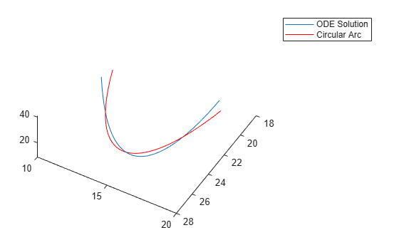
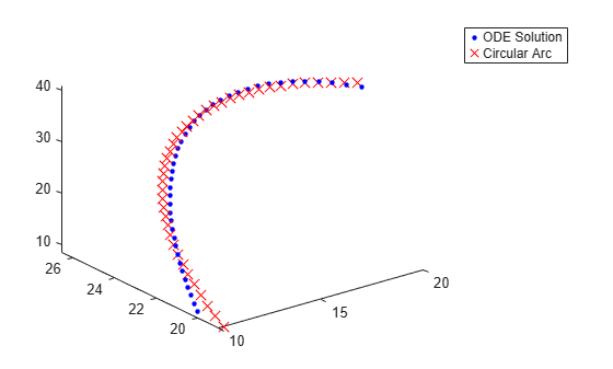
figure
plot3(a(:,1),a(:,2),a(:,3),"b.",MarkerSize=10)
hold on
plot3(soln(:,1),soln(:,2),soln(:,3),"rx",MarkerSize=10)
legend("ODE Solution","Circular Arc")
hold off

원호에 ODE 피팅하기

이제 원호에 최적으로 피팅되도록 파라미터 $$\sigma ,\beta ,and\rho$$를 수정합니다. 더 나은 피팅을 위해 초기점 [10,20,10]도 변경할 수 있도록 합니다.

그렇게 하려면 ODE 피팅의 파라미터를 받아 시간 t에서 궤적을 계산하는 함수 paramfun을 사용하십시오.

function pos = paramfun(x,tspan)

sigma = x(1);
beta = x(2);
rho = x(3);
xt0 = x(4:6);
f = @(t,a) [-sigma*a(1) + sigma*a(2); rho*a(1) - a(2) - a(1)*a(3); -beta*a(3) + a(1)*a(2)];
[~,pos] = ode45(f,tspan,xt0);
end

최적의 파라미터를 구하려면 lsqcurvefit을 사용하여 새로 계산된 ODE 궤적과 원호 soln 간의 차이를 최소화하십시오.

xt0 = zeros(1,6);
xt0(1) = sigma;
xt0(2) = beta;
xt0(3) = rho;
xt0(4:6) = soln(1,:);
[pbest,presnorm,presidual,exitflag,output] = lsqcurvefit(@paramfun,xt0,tspan,soln);

Local minimum possible.

lsqcurvefit stopped because the final change in the sum of squares relative to 
its initial value is less than the value of the function tolerance.

<stopping criteria details>

이 최적화로 인해 파라미터가 얼마나 변경되었는지 확인합니다.

fprintf("New parameters: %f, %f, %f",pbest(1:3))

New parameters: 9.132446, 2.854998, 27.937986

fprintf("Original parameters: %f, %f, %f",[sigma,beta,rho])

Original parameters: 10.000000, 2.666667, 28.000000

파라미터 sigma와 beta가 약 10% 변경되었습니다.

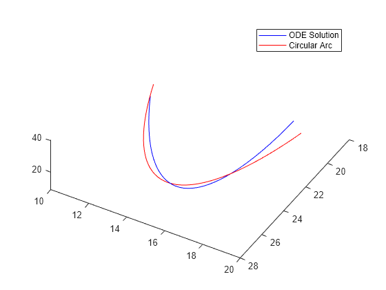
수정된 해를 플로팅합니다.

figure
hold on
odesl = presidual + soln;
plot3(odesl(:,1),odesl(:,2),odesl(:,3),"b")
plot3(soln(:,1),soln(:,2),soln(:,3),"r")
legend("ODE Solution","Circular Arc")
view([-30 -70])
hold off

ODE 피팅의 문제

시뮬레이션 또는 상미분 방정식 최적화하기에서 설명한 바와 같이, 최적화 함수는 수치 ODE 해의 고유한 잡음으로 인해 문제가 있을 수 있습니다. 종료 메시지나 종료 플래그가 잠재적 부정확성을 나타낼 수 있으므로 해가 이상적이지 않다는 의심이 들면 유한 차분을 변경해 보십시오. 이 예제에서 더 큰 유한 차분 스텝 크기와 중심 유한 차분을 사용해 봅니다.

options = optimoptions("lsqcurvefit",FiniteDifferenceStepSize=1e-4,...
    FiniteDifferenceType="central");
[pbest2,presnorm2,presidual2,exitflag2,output2] = ...
    lsqcurvefit(@paramfun,xt0,tspan,soln,[],[],options);

Local minimum possible.

lsqcurvefit stopped because the final change in the sum of squares relative to 
its initial value is less than the value of the function tolerance.

<stopping criteria details>

이 경우에는 이러한 유한 차분 옵션을 사용해도 해가 개선되지는 않습니다.

disp([presnorm,presnorm2])

   20.0637   20.0637

참고 항목

도움말 항목

• Discretized Optimal Trajectory, Problem-Based
• 시뮬레이션 또는 상미분 방정식 최적화하기