Dual Curve Bootstrapping
This example shows how to bootstrap a forward curve using a different curve for discounting.
Define Data
Data is needed for both the forward and discount curve. For this particular example, it is assumed that the data is provided for EONIA (the discount curve) and EURIBOR (the forward curve). However, this approach can be used in any case where the curve to be built is different than the curve used for discounting cash flows. While the data in this example is hardcoded, it could also be imported into MATLAB® with Datafeed Toolbox™ or Database Toolbox™.
Settle = datenum('20-Aug-2013');

% Deposit data
EONIADepositRates = [.0007 .00067]';
EONIADepositMat = datenum({'3-Sep-2013','20-Sep-2013'});
EONIADepositBasis = 2; % act/360
EONIADepositPeriod = 0;

% FRA
EONIAFRARates = [.00025 .0003 .00043 .00054]';
EONIAFRAStartDate = datenum({'11-Sep-2013','9-Oct-2013','13-Nov-2013','11-Dec-2013'});
EONIAFRAEndDate = datenum({'9-Oct-2013','13-Nov-2013','11-Dec-2013','11-Jan-2014'});
EONIAFRABasis = 2; % act/360
EONIAFRAPeriod = 0;

% Swap data
EONIASwapRates = [.0003 .001 .002 .004 .008 .012 .0155 .018 .0193 .02]';
EONIASwapMat = datemnth(Settle,12*[2:5 7 10 15 20 25 30]');
EONIASwapBasis = 5; % 30/360 ISDA
EONIASwapPeriod = 1;

% EURIBOR Deposit data
EURIBORDepositRates = [.0022 .0021 .002 .0019]';
EURIBORDepositMat = datenum({'3-Sep-2013','20-Sep-2013','21-Oct-2013','20-Nov-2013'});
EURIBORDepositBasis = 2; % act/360
EURIBORDepositPeriod = 0;

% EURIBOR Futures
EURIBORFRARates = [9982 9978 9976 9975]';
EURIBORFRAStartDate = datenum({'18-Dec-2013','19-Mar-2014','18-Jun-2014','17-Sep-2014'});
EURIBORFRAEndDate = datenum({'18-Mar-2014','19-Jun-2014','18-Sep-2014','17-Dec-2014'});
EURIBORFRABasis = 2; % act/360
EURIBORFRAPeriod = 4;

% EURIBOR Swap data
EURIBORSwapRates = [.0026 .0044 .0062 .0082 .012 .015 .018 .02 .021 .0215]';
EURIBORSwapMat = datemnth(Settle,12*[2:5 7 10 15 20 25 30]');
EURIBORSwapBasis = 5; % 30/360 ISDA
EURIBORSwapPeriod = 1;
Create EONIA Discount Curve
Build the EONIA curve. This is essentially the same as the single curve case.
CurveType = 'zero';
CurveCompounding = 1;
CurveBasis = 3; % act/365

nEONIADeposits = length(EONIADepositMat);
nEONIAFRA = length(EONIAFRAEndDate);
nEONIASwaps = length(EONIASwapMat);

EONIAInstrumentTypes = [repmat({'deposit'},nEONIADeposits,1);
    repmat({'fra'},nEONIAFRA,1);repmat({'swap'},nEONIASwaps,1)];

EONIAPeriod = [repmat(EONIADepositPeriod,nEONIADeposits,1);
    repmat(EONIAFRAPeriod,nEONIAFRA,1);repmat(EONIASwapPeriod,nEONIASwaps,1)];

EONIABasis = [repmat(EONIADepositBasis,nEONIADeposits,1);
    repmat(EONIAFRABasis,nEONIAFRA,1);repmat(EONIASwapBasis,nEONIASwaps,1)];

EONIAInstrumentData = [[repmat(Settle,[nEONIADeposits 1]);EONIAFRAStartDate;repmat(Settle,[nEONIASwaps 1])] ...
    [EONIADepositMat;EONIAFRAEndDate;EONIASwapMat] ...
    [EONIADepositRates;EONIAFRARates;EONIASwapRates]];

EONIACurve = IRDataCurve.bootstrap(CurveType,Settle,EONIAInstrumentTypes, ...
    EONIAInstrumentData,'Compounding',CurveCompounding,'Basis',CurveBasis, ...
    'InstrumentPeriod',EONIAPeriod,'InstrumentBasis',EONIABasis)
EONIACurve =
			 Type: zero
		   Settle: 735466 (20-Aug-2013)
	  Compounding: 1
			Basis: 3 (actual/365)
	 InterpMethod: linear
			Dates: [16x1 double]
			 Data: [16x1 double]
Create EURIBOR Forward Curve
The EURIBOR forward curve is built first using a single curve approach.
nEURIBORDeposits = length(EURIBORDepositMat);
nEURIBORFRA = length(EURIBORFRAEndDate);
nEURIBORSwaps = length(EURIBORSwapMat);

EURIBORInstrumentTypes = [repmat({'deposit'},nEURIBORDeposits,1);
    repmat({'futures'},nEURIBORFRA,1);repmat({'swap'},nEURIBORSwaps,1)];

EURIBORPeriod = [repmat(EURIBORDepositPeriod,nEURIBORDeposits,1);
    repmat(EURIBORFRAPeriod,nEURIBORFRA,1);repmat(EURIBORSwapPeriod,nEURIBORSwaps,1)];

EURIBORBasis = [repmat(EURIBORDepositBasis,nEURIBORDeposits,1);
    repmat(EURIBORFRABasis,nEURIBORFRA,1);repmat(EURIBORSwapBasis,nEURIBORSwaps,1)];

EURIBORInstrumentData = [repmat(Settle,size(EURIBORInstrumentTypes)) ...
    [EURIBORDepositMat;EURIBORFRAEndDate;EURIBORSwapMat] ...
    [EURIBORDepositRates;EURIBORFRARates;EURIBORSwapRates]];

EURIBORCurve_Single = IRDataCurve.bootstrap(CurveType,Settle,EURIBORInstrumentTypes, ...
    EURIBORInstrumentData,'Compounding',CurveCompounding,'Basis',CurveBasis, ...
    'InstrumentPeriod',EURIBORPeriod,'InstrumentBasis',EURIBORBasis)
EURIBORCurve_Single = Type: zero Settle: 735466 (20-Aug-2013) Compounding: 1 Basis: 3 (actual/365) InterpMethod: linear Dates: [18x1 double] Data: [18x1 double]
Build EURIBOR Curve with EONIA Curve
Build a curve using the EONIA curve as a discounting curve. To do this, specify the EONIA curve as an optional input argument.
EURIBORCurve = IRDataCurve.bootstrap(CurveType,Settle,EURIBORInstrumentTypes, ...
    EURIBORInstrumentData,'DiscountCurve',EONIACurve,'Compounding', ...
    CurveCompounding,'Basis',CurveBasis,'InstrumentPeriod',EURIBORPeriod, ...
    'InstrumentBasis',EURIBORBasis)
EURIBORCurve =
			 Type: zero
		   Settle: 735466 (20-Aug-2013)
	  Compounding: 1
			Basis: 3 (actual/365)
	 InterpMethod: linear
			Dates: [18x1 double]
			 Data: [18x1 double]
Plot Results
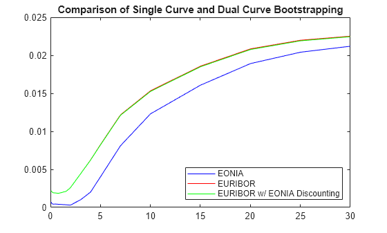
Plot the results to compare the curves.
PlottingDates = (Settle+20:30:Settle+365*30)';
TimeToMaturity = yearfrac(Settle,PlottingDates);

figure
plot(TimeToMaturity, getZeroRates(EONIACurve, PlottingDates),'b')
hold on
plot(TimeToMaturity, getZeroRates(EURIBORCurve_Single, PlottingDates),'r')
plot(TimeToMaturity, getZeroRates(EURIBORCurve, PlottingDates),'g')
title('Comparison of Single Curve and Dual Curve Bootstrapping')
legend({'EONIA','EURIBOR','EURIBOR w/ EONIA Discounting'},'location','southeast')

As expected, the difference between the two different EURIBOR curves is small but nontrivial.
References
This example draws from the following papers and journal articles:
[1] Ametrano, F, and Bianchetti, M. Everything You Always Wanted to Know About Multiple Interest Rate Curve Bootstrapping but Were Afraid to Ask. (April 2, 2013), available at: https://papers.ssrn.com/sol3/papers.cfm?abstract_id=2219548.
[2] Bianchetti, M. Two Curves, One Price. Risk Magazine, pages 74–80, August 2010.
[3] Fujii, M, Shimada, Y, Takahashi, A. A Note on Construction of Multiple Swap Curves with and without Collateral. (January 2, 2010), CARF Working Paper Series No. CARF-F-154, available at: https://papers.ssrn.com/sol3/papers.cfm?abstract_id=1440633.
[4] Mercurio, Fabio. Interest Rates and The Credit Crunch: New Formulas and Market Models. (February 5, 2009), Bloomberg Portfolio Research Paper No. 2010-01-FRONTIERS.
[5] Nashikkar, A. Understanding OIS Discounting., Barclays Capital Interest Rate Strategy, February 24, 2011.
See Also
IRDataCurve | bootstrap | floatbyzero | swapbyzero | getZeroRates
Topics
- Creating Interest-Rate Curve Objects
- Bootstrapping a Swap Curve
- Fitting Interest-Rate Curve Functions
- Interest-Rate Curve Objects and Workflow
- Mapping Financial Instruments Toolbox Curve Functions to Object-Based Framework