Hedge Using Monte Carlo Simulation

Open Live Script

This example shows how to use Monte Carlo simulation to model the probability of different outcomes in a process that cannot easily be predicted due to the intervention of random variables.

Define Stock Profile

Assume the following specification for a stock.

% Price at time 0
Price_0 = 200;

% Drift (annualized)
Drift = 0.08;

% Volatility (annualized)
Vol = 0.4;

% Valuation date
Valuation = '01-Jan-2012';

% Investment horizon date
Horizon = '01-Jan-2013';

% Risk free rate
RiskFreeRate = 0.03;

Use Monte Carlo Simulation

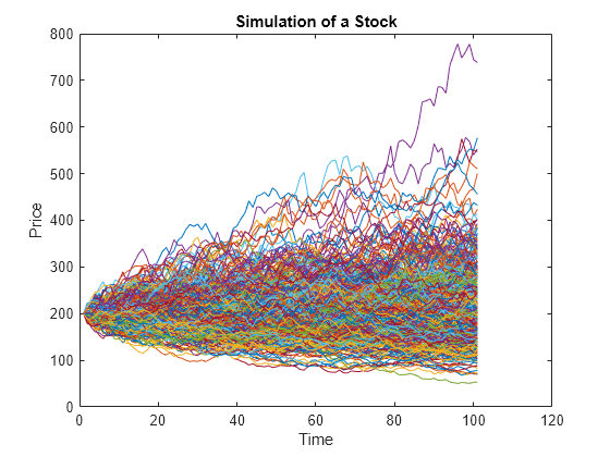
Simulate this stock's price movements from the valuation date to the Horizon date.

% Number of trials for the Monte Carlo simulation
NTRIALS = 100000;

% Length (in years) of the simulation
T = date2time(Valuation,Horizon,1,1);

% Number of periods per trial. Approximately 100 periods per year.
NPERIODS = round(100*T);

% Length (in years) of each time step per period
dt = T/NPERIODS;

% Instantiate the GBM object
StockGBM = gbm(Drift,Vol,'StartState',Price_0);

% Run the simulation
Paths = StockGBM.simByEuler(NPERIODS,'NTRIALS',NTRIALS, ...
    'DeltaTime',dt,'Antithetic',true);

Plot Stock Simulation

For efficiency, only plot some scenarios.

plot(squeeze(Paths(:,:,1:500)));
title('Simulation of a Stock');
xlabel('Time');
ylabel('Price');

Figure contains an axes object. The axes object with title Simulation of a Stock, xlabel Time, ylabel Price contains 500 objects of type line.

Calculate Put Option for Stock Using Black-Scholes

Use blsprice to calculate the put option.

Strike = 190;
[~,Put] = blsprice(Price_0,Strike,RiskFreeRate,T,Vol);

Generate Simulation Matrix

The simulation uses two strategies: (1) stock only and (2) stock with put cover.

AssetScenarios = zeros(NTRIALS,2);
Price_T = squeeze(Paths(end,1,:));

% Strategy 1: Stock only
AssetScenarios(:,1) = (Price_T - Price_0) ./ Price_0

AssetScenarios = 100000×2

    0.5927         0
   -0.4069         0
   -0.2526         0
    0.3365         0
   -0.3606         0
    0.5549         0
   -0.2211         0
    0.3080         0
    0.0849         0
   -0.0416         0
      ⋮

% Strategy 2: Stock with put option cover
AssetScenarios(:, 2) = (max(Price_T, Strike) - (Price_0 + Put)) ./ ...
    (Price_0 + Put)

AssetScenarios = 100000×2

    0.5927    0.4266
   -0.4069   -0.1490
   -0.2526   -0.1490
    0.3365    0.1972
   -0.3606   -0.1490
    0.5549    0.3928
   -0.2211   -0.1490
    0.3080    0.1716
    0.0849   -0.0282
   -0.0416   -0.1415
      ⋮

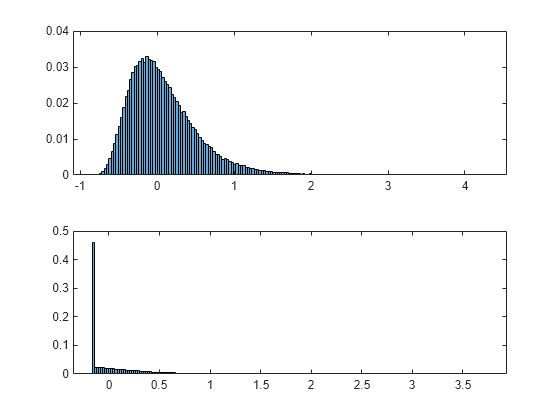
Plot Distributions

The returns for the two strategies are not normally distributed.

% Create histogram
figure;
subplot(2,1,1);
histogram(AssetScenarios(:,1),'Normalization','probability')
subplot(2,1,2);
histogram(AssetScenarios(:,2),'Normalization','probability')

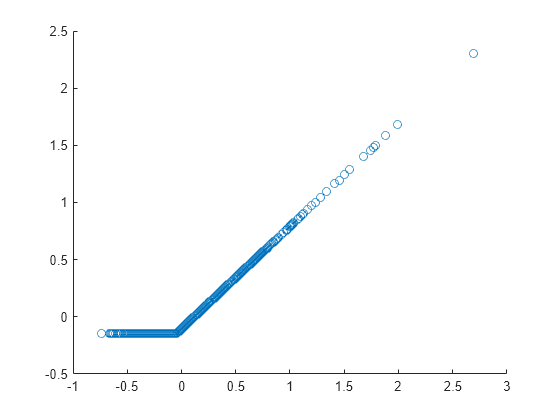
Figure contains 2 axes objects. Axes object 1 contains an object of type histogram. Axes object 2 contains an object of type histogram.

% Create scatter plot of the two strategies. Notice that the two strategies are highly
% correlated.
figure;
scatter(AssetScenarios(1:1000,1),AssetScenarios(1:1000,2));

Figure contains an axes object. The axes object contains an object of type scatter.

Create PortfolioCVaR Object to Obtain Portfolio Weights

Create a PortfolioCVaR object.

p = PortfolioCVaR('Scenarios',AssetScenarios,'LowerBound',0, ...
    'Budget',1,'ProbabilityLevel',0.95)

p = 
  PortfolioCVaR with properties:

                       BuyCost: []
                      SellCost: []
                  RiskFreeRate: []
              ProbabilityLevel: 0.9500
                      Turnover: []
                   BuyTurnover: []
                  SellTurnover: []
                  NumScenarios: 100000
                          Name: []
                     NumAssets: 2
                     AssetList: []
                      InitPort: []
                   AInequality: []
                   bInequality: []
                     AEquality: []
                     bEquality: []
                    LowerBound: [2x1 double]
                    UpperBound: []
                   LowerBudget: 1
                   UpperBudget: 1
                   GroupMatrix: []
                    LowerGroup: []
                    UpperGroup: []
                        GroupA: []
                        GroupB: []
                    LowerRatio: []
                    UpperRatio: []
                  MinNumAssets: []
                  MaxNumAssets: []
    ConditionalBudgetThreshold: []
        ConditionalUpperBudget: []
                     BoundType: []

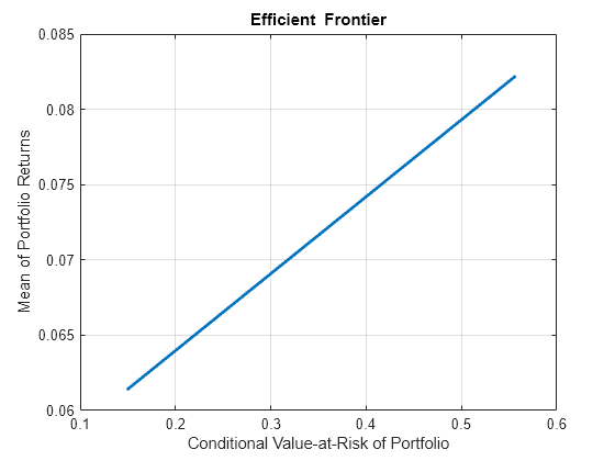
% Estimate the efficient frontier to obtain portfolio weights
pwgt = estimateFrontier(p);

% Plot the efficient frontier
figure;
plotFrontier(p,pwgt);

Figure contains an axes object. The axes object with title Efficient Frontier, xlabel Conditional Value-at-Risk of Portfolio, ylabel Mean of Portfolio Returns contains an object of type line. This object represents Efficient Frontier.

% Plot the portfolio weights
figure;
area(pwgt');
axis([1 10 0 1])
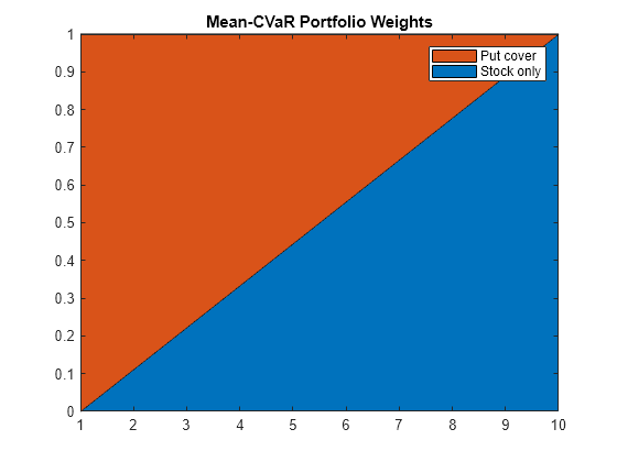
legend('Stock only','Put cover');
title('Mean-CVaR Portfolio Weights');

Figure contains an axes object. The axes object with title Mean-CVaR Portfolio Weights contains 2 objects of type area. These objects represent Stock only, Put cover.

Add Hedging Strategies

Use blsprice to calculate prices of put options with different strikes.

% Put option with strike at 50% of current underlying price
Strike50 = 0.50*Price_0;
[~, Put50] = blsprice(Price_0,Strike50,RiskFreeRate,T,Vol);

% Put option with strike at 75% of current underlying price
Strike75 = 0.75*Price_0;
[~, Put75] = blsprice(Price_0,Strike75,RiskFreeRate,T,Vol);

% Put option with strike at 90% of current underlying price
Strike90 = 0.90*Price_0;
[~, Put90] = blsprice(Price_0,Strike90,RiskFreeRate,T,Vol);

% Put option with strike at 95% of current underlying price
Strike95 = 0.95*Price_0; % Same as strike
[~, Put95] = blsprice(Price_0,Strike95,RiskFreeRate,T,Vol);

Generate Simulation Matrix for Strategies

Generate simulation matrix for the strategy variations.

AssetScenarios = zeros(NTRIALS, 5);

% Strategy 1: Stock only
AssetScenarios(:, 1) = (Price_T - Price_0) ./ Price_0;

% Strategy 2: Put option cover at 50%
AssetScenarios(:, 2) = (max(Price_T, Strike50) - (Price_0 + Put50)) ./ ...
    (Price_0 + Put50);

% Strategy 2: Put option cover at 75%
AssetScenarios(:, 3) = (max(Price_T, Strike75) - (Price_0 + Put75)) ./ ...
    (Price_0 + Put75);

% Strategy 2: Put option cover at 90%
AssetScenarios(:, 4) = (max(Price_T, Strike90) - (Price_0 + Put90)) ./ ...
    (Price_0 + Put90);

% Strategy 2: Put option cover at 95%
AssetScenarios(:, 5) = (max(Price_T, Strike95) - (Price_0 + Put95)) ./ ...
    (Price_0 + Put95);

Create PortfolioCVar Object Using Hedging Strategies

Create a PortfolioCVaR object using the hedging strategies.

p = PortfolioCVaR('Name','CVaR Portfolio Five Hedging Levels', ...
   'AssetList',{'Stock','Hedge50','Hedge75','Hedge90','Hedge95'}, ...
   'Scenarios',AssetScenarios,'LowerBound',0, ...
   'Budget',1,'ProbabilityLevel',0.95);

% Estimate the efficient frontier to obtain portfolio weights
pwgt = estimateFrontier(p);

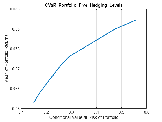
% Plot the efficient frontier
figure;
plotFrontier(p,pwgt);

Figure contains an axes object. The axes object with title CVaR Portfolio Five Hedging Levels, xlabel Conditional Value-at-Risk of Portfolio, ylabel Mean of Portfolio Returns contains an object of type line. This object represents Efficient Frontier.

% Plot the portfolio weights
figure;
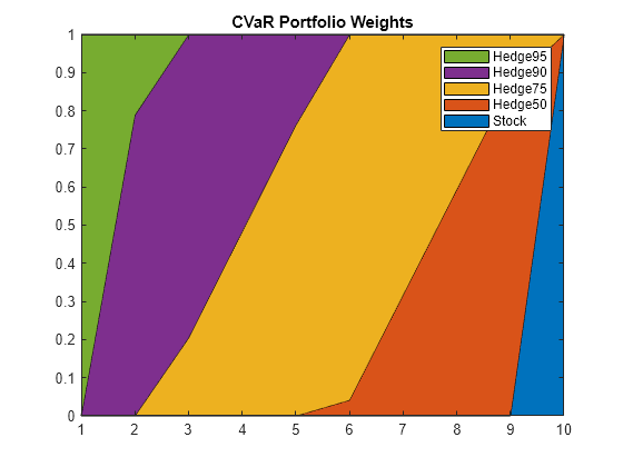
area(pwgt');
legend(p.AssetList);
axis([1 10 0 1])
title('CVaR Portfolio Weights');

Figure contains an axes object. The axes object with title CVaR Portfolio Weights contains 5 objects of type area. These objects represent Stock, Hedge50, Hedge75, Hedge90, Hedge95.

Create Mean-Variance Portfolio

Create a Portfolio object to compare with the PortfolioCVaR object.

% Create the Portfolio object
pmv = Portfolio('Name','Mean-Variance Portfolio Five Hedging Levels', ...
   'AssetList',{'Stock','Hedge50','Hedge75','Hedge90','Hedge95'});
pmv = pmv.estimateAssetMoments(p.getScenarios);
pmv = pmv.setDefaultConstraints;

% Estimate the efficient frontier to obtain portfolio weights
pwgtmv = pmv.estimateFrontier;

% Plot the efficient frontier
figure;
mvFrontierHandle = pmv.plotFrontier(pwgtmv);

Figure contains an axes object. The axes object with title Mean-Variance Portfolio Five Hedging Levels, xlabel Standard Deviation of Portfolio Returns, ylabel Mean of Portfolio Returns contains an object of type line. This object represents Efficient Frontier.

% Plot the portfolio weights
figure;
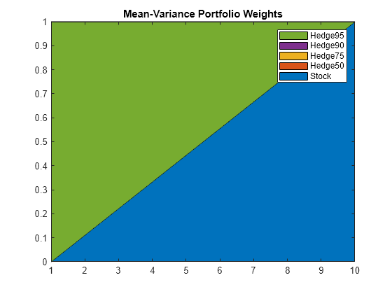
area(pwgtmv');
legend(pmv.AssetList);
axis([1 10 0 1])
title('Mean-Variance Portfolio Weights');

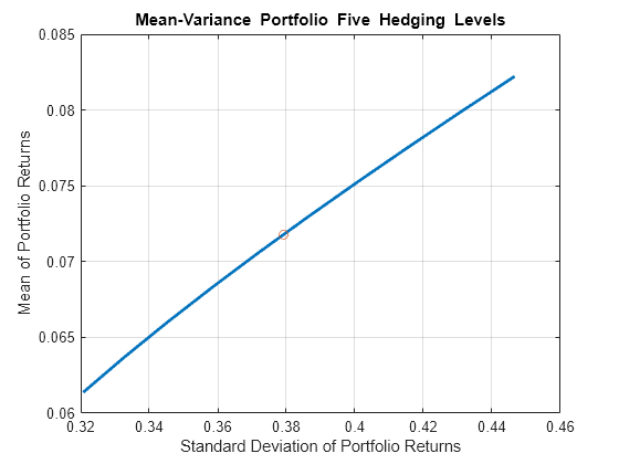
Figure contains an axes object. The axes object with title Mean-Variance Portfolio Weights contains 5 objects of type area. These objects represent Stock, Hedge50, Hedge75, Hedge90, Hedge95.

Plot Target Portfolio on Mean Variance Frontier

Determine the achievable levels of return.

% Achievable levels of return
pretlimits = pmv.estimatePortReturn(pmv.estimateFrontierLimits);
TargetRet = mean(pretlimits); % Target half way up the frontier

% Obtain risk level at target return
pwgtmvTarget = pmv.estimateFrontierByReturn(TargetRet);
priskTarget = pmv.estimatePortRisk(pwgtmvTarget);

% Plot point onto mean variance frontier
figure;
pmv.plotFrontier(pwgtmv);
hold on
scatter(priskTarget,TargetRet);
hold off

Figure contains an axes object. The axes object with title Mean-Variance Portfolio Five Hedging Levels, xlabel Standard Deviation of Portfolio Returns, ylabel Mean of Portfolio Returns contains 2 objects of type line, scatter. This object represents Efficient Frontier.

Plot Mean Variance Efficient Portfolio on CVaR Frontier

The following plot displays that the target portfolio is below the mean-CVaR efficient frontier.

% Obtain CVaR risk for mean variance target return portfolio
pretTargetCVaR = p.estimatePortReturn(pwgtmvTarget); % Should be TargetRet
priskTargetCVaR = p.estimatePortRisk(pwgtmvTarget);  % Risk proxy is CVaR

% Plot target return portfolio onto mean-CVaR frontier
figure;
p.plotFrontier(pwgt);
hold on
scatter(priskTargetCVaR,pretTargetCVaR);
hold off

Figure contains an axes object. The axes object with title CVaR Portfolio Five Hedging Levels, xlabel Conditional Value-at-Risk of Portfolio, ylabel Mean of Portfolio Returns contains 2 objects of type line, scatter. This object represents Efficient Frontier.