피팅 미분 및 적분하기
이 예제에서는 예측 변수 값에서 피팅의 1계 및 2계 도함수와 피팅의 적분을 구하는 방법을 보여줍니다.
기준 정현파 신호를 만듭니다.
xdata = (0:.1:2*pi)';
y0 = sin(xdata);
신호에 잡음을 추가합니다.
noise = 2*y0.*randn(size(y0)); % Response-dependent noise
ydata = y0 + noise;
잡음이 있는 데이터를 사용자 지정 정현파 모델로 피팅합니다.
f = fittype('a*sin(b*x)');
fit1 = fit(xdata,ydata,f,'StartPoint',[1 1]);
예측 변수에서 피팅의 도함수를 구합니다.
[d1,d2] = differentiate(fit1,xdata);
데이터, 피팅 및 도함수를 플로팅합니다.
subplot(3,1,1)
plot(fit1,xdata,ydata) % cfit plot method
subplot(3,1,2)
plot(xdata,d1,'m') % double plot method
grid on
legend('1st derivative')
subplot(3,1,3)
plot(xdata,d2,'c') % double plot method
grid on
legend('2nd derivative')
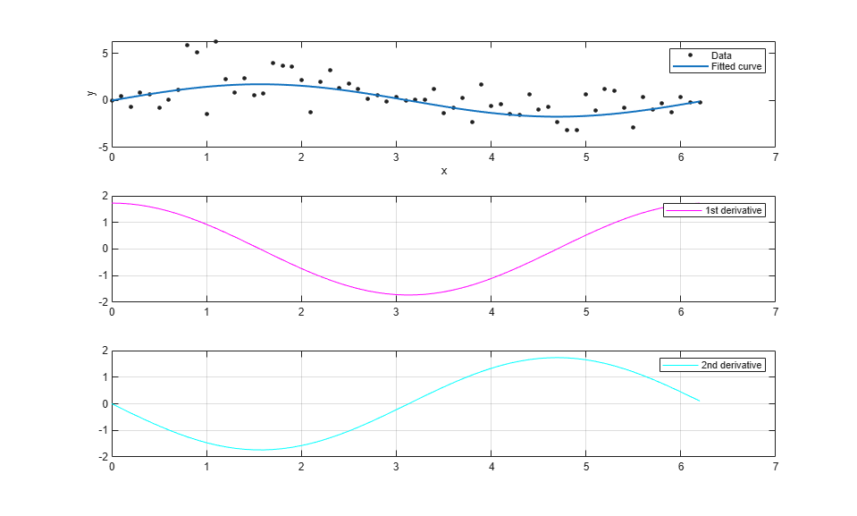
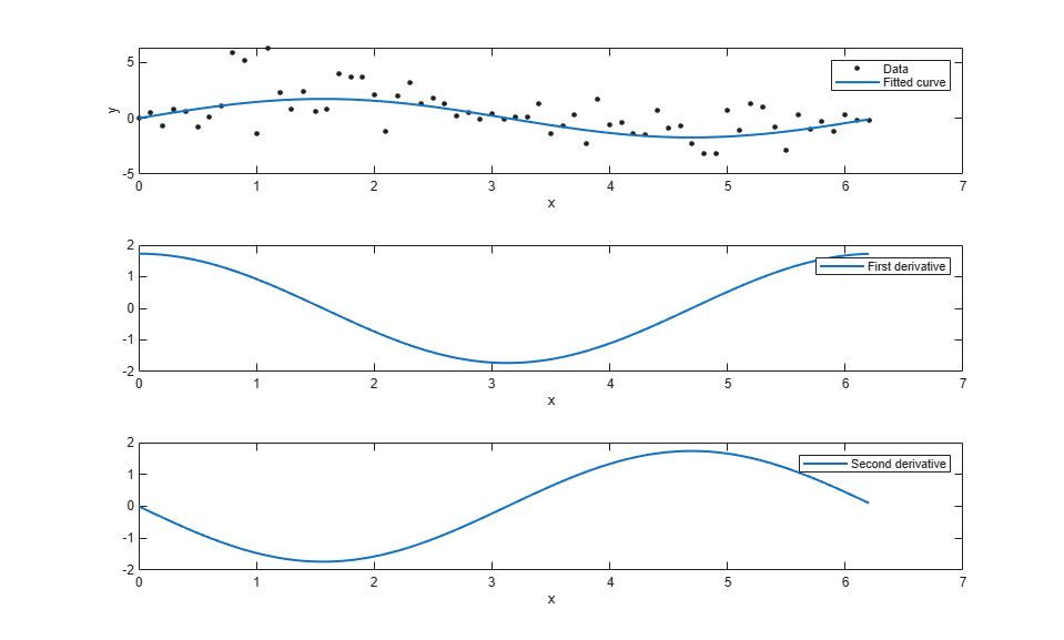
도함수는 다음과 같이 cfit plot 메서드로 직접 계산하고 플로팅할 수도 있습니다. 그러나 plot 메서드는 도함수에 대한 데이터를 반환하지 않습니다.
plot(fit1,xdata,ydata,{'fit','deriv1','deriv2'})
예측 변수에서 피팅의 적분을 구합니다.
int = integrate(fit1,xdata,0);
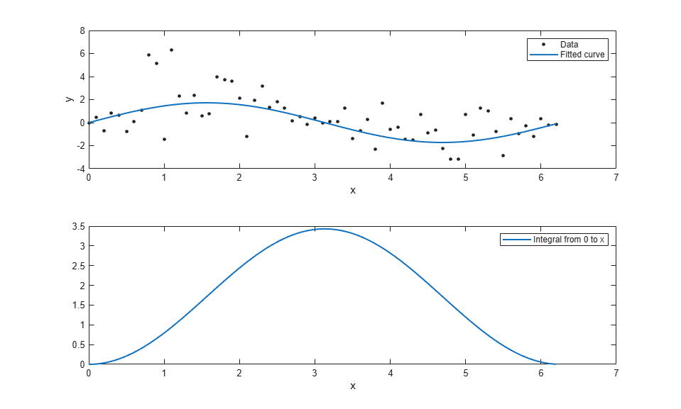
데이터, 피팅 및 적분을 플로팅합니다.
subplot(2,1,1)
plot(fit1,xdata,ydata) % cfit plot method
subplot(2,1,2)
plot(xdata,int,'m') % double plot method
grid on
legend('integral')
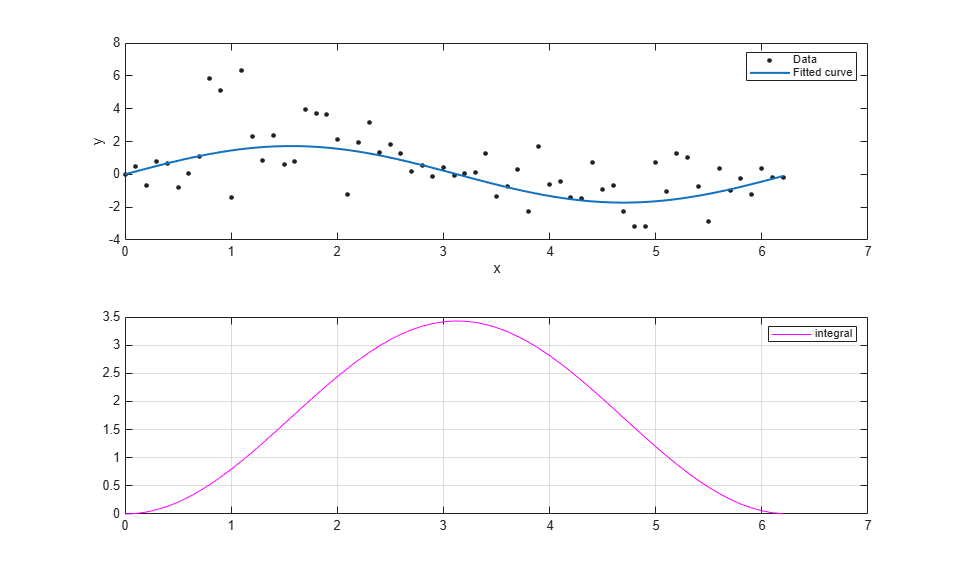
적분은 다음과 같이 cfit plot 메서드로 직접 계산하고 플로팅할 수도 있습니다. 그러나 plot 메서드는 적분에 대한 데이터를 반환하지 않습니다.
plot(fit1,xdata,ydata,{'fit','integral'})