올림 코사인 필터링
이 예제에서는 올림 코사인 필터의 심볼간 간섭(ISI) 제거 기능과, 올림 코사인 송신 필터 및 수신 필터 System object를 사용하여 송신기와 수신기 간에 올림 코사인 필터링을 분리하는 방법을 보여줍니다.
올림 코사인 필터 사양
올림 코사인 필터의 기본 파라미터는 필터의 대역폭을 간접적으로 지정하는 롤오프 인자입니다. 이상적인 올림 코사인 필터의 탭 개수는 무한합니다. 따라서 실제 올림 코사인 필터에는 윈도우가 적용됩니다. 윈도우 길이는 FilterSpanInSymbols 속성을 사용하여 제어됩니다. 이 예제에서는 필터가 6개의 심볼 지속 시간에 걸쳐 있기 때문에 윈도우 길이를 6개의 심볼 지속 시간으로 지정합니다. 이러한 필터는 3개 심볼 지속 시간의 군지연도 갖습니다. 올림 코사인 필터는 신호가 업샘플링되는 펄스 성형에 사용됩니다. 따라서 업샘플링 인자도 지정해야 합니다. 이 예제에서는 올림 코사인 필터를 설계하는 데 다음 파라미터를 사용합니다.
% Define the parameters
Nsym = 6;                                 % Filter span in symbol durations
beta = [0.1, 0.3, 0.5, 0.7, 0.9];         % Roll-off factor
sampsPerSym = 8;                          % Upsampling factor
colors = ["r", "g", "b", "c", "m"];       % Define colors for different beta values
각 베타 값에 대해 올림 코사인 송신 필터 System object™를 만들고 그 속성을 설정하여 원하는 필터 특성을 얻습니다. impz를 사용하여 필터 특성을 시각화합니다. 올림 코사인 송신 필터 System object는 단위 에너지를 갖는 Direct-Form 다상 FIR 필터를 설계합니다. 이 필터의 차수는 Nsym*sampsPerSym입니다(혹은 Nsym*sampsPerSym+1 개의 탭을 가집니다). Gain 속성을 활용하여 필터 계수를 정규화하여 필터링된 데이터와 필터링되지 않은 데이터를 중첩했을 때 두 데이터가 일치하도록 할 수 있습니다.
% Create figures for plotting
figure(Name="Unnormalized Impulse Responses");
hold on;
figure(Name="Normalized Impulse Responses");
hold on;

for i = 1:length(beta)
    % Create a raised cosine transmit filter for each beta value
    rctFilt = comm.RaisedCosineTransmitFilter(RolloffFactor=beta(i), ...
        FilterSpanInSymbols=Nsym, ...
        OutputSamplesPerSymbol=sampsPerSym);

    % Extract the filter coefficients
    b = coeffs(rctFilt);

    % Compute the unnormalized impulse response
    [h_unnorm, t_unnorm] = impz(b.Numerator);

    % Switch to the unnormalized figure to plot
    figure(findobj(Name="Unnormalized Impulse Responses"));
    plot(t_unnorm, h_unnorm, colors(i), Marker="o", ...
        DisplayName=['\beta = ', num2str(beta(i))]);

    % Normalize the filter coefficients
    rctFilt.Gain = 1/max(b.Numerator);

    % Compute the normalized impulse response
    [h_norm, t_norm] = impz(b.Numerator * rctFilt.Gain);

    % Switch to the normalized figure to plot
    figure(findobj(Name="Normalized Impulse Responses"));
    plot(t_norm, h_norm, colors(i), Marker="o", ...
        DisplayName=['\beta = ', num2str(beta(i))]);
end

% The unnormalized figure
figure(findobj(Name="Unnormalized Impulse Responses"));
hold off;
title("Unnormalized Impulse Responses for Different Roll-off Factors");
xlabel("Samples");
ylabel("Amplitude");
legend("show");

figure(findobj('Name', 'Normalized Impulse Responses'));
hold off;
title("Normalized Impulse Responses for Different Roll-off Factors");
xlabel("Samples");
ylabel("Amplitude");
legend show;

올림 코사인 필터로 펄스 성형
양극성 데이터 시퀀스를 생성하고 올림 코사인 필터를 사용하여 ISI가 없는 파형을 성형합니다.
% Parameters
DataL = 20;             % Data length in symbols
R = 1000;               % Data rate
Fs = R * sampsPerSym;   % Sampling frequency

% Create a local random stream to be used by random number generators for
% repeatability
hStr = RandStream('mt19937ar',Seed=0);

% Generate random data
x = 2*randi(hStr,[0 1],DataL,1)-1;
% Time vector sampled at symbol rate in milliseconds
tx = 1000 * (0: DataL - 1) / R;
플롯에서 디지털 데이터와 보간된 신호를 비교합니다. 필터의 피크 응답이 필터의 군지연(Nsym/(2*R))에 의해 지연되기 때문에 두 신호를 비교하기가 어렵습니다. 입력값 x 끝에 Nsym/2개의 0을 추가하여 모든 유용한 샘플을 필터에서 플러시합니다.
% Design raised cosine filter with given order in symbols
rctFilt1 = comm.RaisedCosineTransmitFilter(...
  Shape='Normal', ...
  RolloffFactor=0.5, ...
  FilterSpanInSymbols=Nsym, ...
  OutputSamplesPerSymbol=sampsPerSym);


% Normalize to obtain maximum filter tap value of 1
b1 = coeffs(rctFilt1);
rctFilt1.Gain = 1/max(b1.Numerator);

% Visualize the impulse response
%impz(rctFilt.coeffs.Numerator)

% Filter
yo = rctFilt1([x; zeros(Nsym/2,1)]);
% Time vector sampled at sampling frequency in milliseconds
to = 1000 * (0: (DataL+Nsym/2)*sampsPerSym - 1) / Fs;
% Plot data
fig1 = figure;
stem(tx, x, 'kx'); hold on;
% Plot filtered data
plot(to, yo, 'b-'); hold off;
% Set axes and labels
axis([0 30 -1.7 1.7]);  xlabel('Time (ms)'); ylabel('Amplitude');
legend('Transmitted data','Upsampled data','Location','southeast')

입력 신호를 지연시켜 올림 코사인 필터 군지연을 보정합니다. 이제 올림 코사인 필터가 어떻게 신호를 업샘플링하고 필터링하는지 쉽게 볼 수 있습니다. 필터링된 신호가 입력 샘플 시간에서 지연된 입력 신호와 동일합니다. 이 결과는 올림 코사인 필터가 신호 대역을 제한하면서 동시에 ISI를 방지할 수 있다는 것을 보여줍니다.
% Filter group delay, since raised cosine filter is linear phase and
% symmetric.
fltDelay = Nsym / (2*R);
% Correct for propagation delay by removing filter transients
yo = yo(fltDelay*Fs+1:end);
to = 1000 * (0: DataL*sampsPerSym - 1) / Fs;
% Plot data.
stem(tx, x, 'kx'); hold on;
% Plot filtered data.
plot(to, yo, 'b-'); hold off;
% Set axes and labels.
axis([0 25 -1.7 1.7]);  xlabel('Time (ms)'); ylabel('Amplitude');
legend('Transmitted data','Upsampled data','Location','southeast')

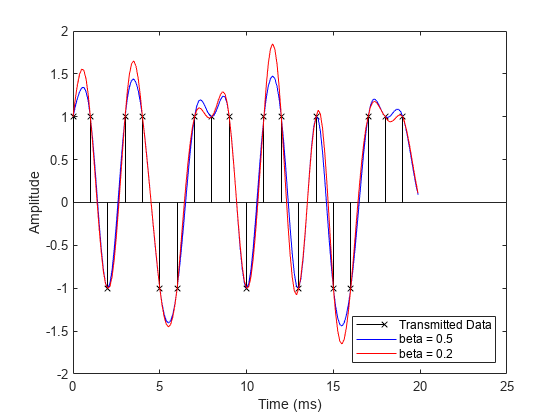
롤오프 인자
롤오프 인자를 0.5(파란색 곡선)에서 0.2(빨간색 곡선)로 변경했을 때 필터링된 출력에 미치는 영향을 확인해 봅니다. 롤오프 값이 낮을수록 필터의 천이 대역이 좁아지기 때문에 필터링된 신호의 오버슈트가 파란색 곡선보다 빨간색 곡선에서 더 큽니다.
% Set roll-off factor to 0.2
rctFilt2 = comm.RaisedCosineTransmitFilter(...
  Shape='Normal', ...
  RolloffFactor=0.2, ...
  FilterSpanInSymbols=Nsym, ...
  OutputSamplesPerSymbol=sampsPerSym);
% Normalize filter
b = coeffs(rctFilt2);
rctFilt2.Gain = 1/max(b.Numerator);
% Filter
yo1 = rctFilt2([x; zeros(Nsym/2,1)]);
% Correct for propagation delay by removing filter transients
yo1 = yo1(fltDelay*Fs+1:end);
% Plot data
stem(tx, x, 'kx'); hold on;
% Plot filtered data
plot(to, yo, 'b-',to, yo1, 'r-'); hold off;
% Set axes and labels
axis([0 25 -2 2]);  xlabel('Time (ms)'); ylabel('Amplitude');
legend('Transmitted Data','beta = 0.5','beta = 0.2', ...
    'Location','southeast')
제곱근 올림 코사인 필터
올림 코사인 필터링은 일반적으로 송신기와 수신기 간에 필터링을 분리하는 데 사용됩니다. 송신기와 수신기 모두 제곱근 올림 코사인 필터를 사용합니다. 송신기 필터와 수신기 필터를 결합한 것이 올림 코사인 필터이기 때문에 최소한의 ISI가 발생합니다. 형태를 'Square root'로 설정하여 제곱근 올림 코사인 필터를 지정합니다.
% Design raised cosine filter with given order in symbols
rctFilt3 = comm.RaisedCosineTransmitFilter(...
  Shape="Square root", ...
  RolloffFactor=0.5, ...
  FilterSpanInSymbols=Nsym, ...
  OutputSamplesPerSymbol=sampsPerSym);
설계된 필터를 사용하여 송신기에서 데이터를 업샘플링하고 필터링합니다. 다음 플롯은 제곱근 올림 코사인 필터를 사용하여 필터링해서 송신된 신호를 보여줍니다.
% Upsample and filter.
yc = rctFilt3([x; zeros(Nsym/2,1)]);
% Correct for propagation delay by removing filter transients
yc = yc(fltDelay*Fs+1:end);
% Plot data.
stem(tx, x, 'kx'); hold on;
% Plot filtered data.
plot(to, yc, 'm-'); hold off;
% Set axes and labels.
axis([0 25 -1.7 1.7]);  xlabel('Time (ms)'); ylabel('Amplitude');
legend('Transmitted data','Sqrt. raised cosine','Location','southeast')

그런 다음 수신기에서 송신된 신호(자홍색 곡선)를 필터링합니다(전체 파형을 표시하기 위해 필터 출력을 데시메이션하지 않음). 디폴트 단위 에너지 정규화를 수행하면 송신 필터와 수신 필터를 결합한 이득이 정규화된 올림 코사인 필터의 이득과 동일하게 됩니다. (수신기에서 파란색 곡선으로 표시된) 필터링된 수신 신호가 하나의 올림 코사인 필터를 사용하여 필터링된 신호와 거의 동일합니다.
% Design and normalize filter.
rcrFilt = comm.RaisedCosineReceiveFilter(...
  'Shape',                  'Square root', ...
  'RolloffFactor',          0.5, ...
  'FilterSpanInSymbols',    Nsym, ...
  'InputSamplesPerSymbol',  sampsPerSym, ...
  'DecimationFactor',       1);
% Filter at the receiver.
yr = rcrFilt([yc; zeros(Nsym*sampsPerSym/2, 1)]);
% Correct for propagation delay by removing filter transients
yr = yr(fltDelay*Fs+1:end);
% Plot data.
stem(tx, x, 'kx'); hold on;
% Plot filtered data.
plot(to, yr, 'b-',to, yo, 'm:'); hold off;
% Set axes and labels.
axis([0 25 -1.7 1.7]);  xlabel('Time (ms)'); ylabel('Amplitude');
legend('Transmitted Data','Received filter output', ...
    'Raised cosine filter output','Location','southeast')

롤오프 인자가 단일 반송파 시스템의 PAPR에 미치는 영향
PAPR(피크 대 평균 전력 비율)은 신호의 피크가 평균 전력 수준에 비해 얼마나 큰지를 정량화하는 척도입니다. PAPR이 높다는 것은 신호가 때때로 평균 전력에 비해 매우 높은 피크 값을 갖는다는 것을 나타내는데, 이는 전력 증폭기에 부담을 주고 비선형 왜곡을 초래합니다.
올림 코사인 필터의 롤오프 인자는 필터의 통과대역에서 저지대역으로의 천이 대역폭을 결정합니다. 롤오프 인자가 작으면 천이가 더 급격해져서 대역폭 사용 효율성은 높아지지만 PAPR이 높아질 가능성이 있습니다. 주파수 영역에서의 급격한 천이는 시간 영역에서 더 높은 피크 진폭으로 이어질 수 있습니다.
반대로, 롤오프 인자가 크면 주파수 영역에서 천이가 더 완만해지고, 신호의 시간 영역 피크가 덜 두드러지기 때문에 PAPR이 낮아집니다. 그러나 이러한 결과는 대역폭 사용량을 증가시키는 부작용을 만듭니다.
이 예제는 단일 반송파 시스템에서 롤오프 인자가 BPSK(이진 위상 편이 변조) 신호의 PAPR에 미치는 영향을 보여줍니다.
N = 10000; % Number of bits
M = 2;     % Modulation order (BPSK in this case)
rolloffFactors = [0.1, 0.15, 0.25, 0.3, 0.35, 0.45];
sampsPerSym = 2;
Nsym = 6;  % Filter span in symbols

% Generate a random binary signal
data = randi([0 M-1], N, 1);

% BPSK Modulation
modData = pskmod(data, M);

% Initialize vector to store PAPR values
paprValues = zeros(length(rolloffFactors), 1);

for i = 1:length(rolloffFactors)
    % Create raised cosine transmit filter
    rctFilt = comm.RaisedCosineTransmitFilter(...
        RolloffFactor=rolloffFactors(i), ...
        FilterSpanInSymbols=Nsym, ...
        OutputSamplesPerSymbol=sampsPerSym);
    % Filter the modulated data
    txSig = rctFilt(modData);
    % Create a powermeter object for PAPR measurement
    meter = powermeter(Measurement="Peak-to-average power ratio", ...
        ComputeCCDF=true);
    % Calculate PAPR
    papr = meter(txSig);
    paprValues(i) = papr;
end

% Plot PAPR vs. roll-off factor
figure;
plot(rolloffFactors, paprValues, '-o');
xlabel("Roll-off Factor");
ylabel("PAPR (dB)");
title("PAPR vs. Roll-off Factor for Raised Cosine Filtered Signals");
grid on;

계산 비용
다음 표에서는 다상 FIR 보간 필터와 다상 FIR 데시메이션 필터의 계산 비용을 비교합니다.
C1 = cost(rctFilt3);
C2 = cost(rcrFilt);
------------------------------------------------------------------------
                    Implementation Cost Comparison
------------------------------------------------------------------------
                        Multipliers  Adders  Mult/Symbol  Add/Symbol
Multirate Interpolator      49         41          49         41
Multirate Decimator         49         48           6.125      6