High Precision Orbit Propagation of the International Space Station
This example shows how to propagate the orbit of the International Space Station (ISS) using high precision numerical orbit propagation with Aerospace Blockset™. It uses the Orbit Propagator block to calculate the ISS trajectory for 24 hours. The example then compares position and velocity states to publicly available ISS trajectory data available from NASA Trajectory Operations and Planning (TOPO) flight controllers at Johnson Space Center.
The Orbit Propagator block models translational dynamics of spacecraft using numerical integration. It computes the position and velocity of one or more spacecraft over time. For the most accurate results, use a variable step solver with low tolerance settings (less than 1e-9). Depending on your mission requirements, you can speed up simulation run time by using larger tolerances. Doing so might impact the accuracy of the solution. To propagate orbital states, the block uses the gravity model selected for the current central body. The block also includes atmospheric drag (for Earth orbits), gravitational effects of celestial bodies other than the central body, and solar radiation pressure. The block also takes into account external perturbing accelerations that you provide as inputs to the block.
In this example, use ISS International Celestial Reference Frame (ICRF) position and velocity states directly from the referenced NASA public distribution file [1] to initialize an ISS orbit in the Orbit Propagator block. Use the EGM2008 spherical harmonic gravity model to model Earth gravity and the NRLMSISE-00 atmospheric model to compute atmospheric drag, including the effects of space weather (solar flux and geomagnetic indices) on atmospheric density. Calculate third body gravity point-mass contributions for the Moon, Sun, Jupiter. Lastly, include effects of solar radiation pressure (SRP) assuming a spherical satellite geometry. Perturbations due to third body gravity and solar radiation pressure are near-negligable in a low Earth orbit like that of the ISS. However, to demostrate possible configurations for high precision orbit propagation, they are included in this example. Perturbations required for accurate trajectory modeling vary depending on the application and orbital regime. Determine which perturbations to include on a case-by-case basis for your mission.
Run the model for 24 hours, and compare against the published NASA trajectory data.
Set Mission Initial Conditions
This example uses MATLAB® structures to organize mission data. These structures make accessing data later in the example more intuitive. They also help declutter the global base workspace.
The referenced ISS ephemeris data file [1] provided by NASA begins on January 3, 2022 at 12:00:00.000 UTC.
mission.StartDate = datetime(2022, 1, 3, 12, 0, 0);
mission.Duration  = hours(24);
The file contains ICRF position (km) and velocity (km/s) data sampled every 4 minutes.
iss.X0_icrf = [-1325.896391725290 5492.890955896010 3762.423747679220]; % km
iss.V0_icrf = [-4.87470128630892  -4.10251688094599 4.26428812476909];  % km/s
It also contains mass (kg), drag area (m^2), and drag coefficient data corresponding with the epoch.
iss.Mass      = 459023.0; % kg
iss.DragArea  = 1951.0;   % m^2
iss.DragCoeff = 2.0;
The file also includes solar radiation area (m^2) and a solar radiation coefficient; however these values are zero because SRP is not prominent in low Earth orbit (LEO) where the ISS operates. Despite their trivial impact on the resultant trajectory, we will include solar radiation pressure calculations in this example to fully demonstrate high precision orbit propagation. SRP is more prominent at higher orbital regimes.
iss.SRPArea  = 1500;         % m^2
iss.SRPCoeff = 1.8;
iss.P_sr     = 4.5344321e-6; % N/m^2
High Precision Orbit Propagation Algorithm
The Orbit Propagator block performs high precision numerical orbit propagation using Cowell's method. To compute the position and velocity at each time step of the simulationn the inertial (ICRF) frame, Earth gravitational acceleration is summed with all perturbating accelerations and double-integrated.
where:
is the acceleration due to Earth gravity.
is the acceleration due to atmospheric drag.
is the acceleration due to gravity of the Moon, Sun, and planets of the solar system. The correct list of third bodies to include depends on the central body, orbit, and application.
is the acceleration due to solar radiation pressure.
Earth Gravity
The gravity model for Earth in this example is the EGM2008 spherical harmonic gravity model. This model accounts for zonal, sectoral, and tesseral harmonics. For reference, the second-degree zeroth order zonal harmonic , which accounts for the oblateness of Earth, is . Spherical Harmonic models accounts for harmonics up to max degree . For EGM2008, .
Spherical harmonic gravity is computed in the fixed frame (ff) coordinated system (International Terrestrial Reference Frame (ITRF), in the case of Earth). Numerical integration, however, is always performed in the inertial ICRF coordinate system. Therefore, at each timestep, position and velocity states are transformed into the fixed-frame, gravity is calculated in the fixed-frame, and the resulting acceleration is transformed into the inertial frame.
where:
given the following partial derivatives in spherical coordinates:
are associated Legendre functions.
and are the unnormalized harmonic coefficients.
Atmospheric Drag
The Orbit Propagator block supports inclusion of acceleration due to atmospheric drag using the NRLMSISE-00 atmosphere model. Atmospheric drag is a dominant perturbation in LEO and causes the ISS orbit to degrade over time without assistance from orbital maneuvers.
Atmospheric drag is calculated as:
where:
is the atmospheric density.
is the spacecraft drag coefficient.
is the spacecraft drag area, or the area normal to .
is the spacecraft mass.
is the spacecraft velocity relative to the atmosphere.
The NRLMSISE-00 atmospheric model is used to calculate atmospheric density. It requires space weather data (F10.7 and F10.7A radio flux values and geomagnetic indices), which can be obtained in a consolidated format from CelesTrak®. For more information about space weather data in MATLAB and Simulink®, see the Solar Flux and Geomagnetic Index block reference page and the Aerospace Toolbox aeroReadSpaceWeatherData function reference page.
Third Body Gravity
Third body gravity can be included in the Orbit Propagator block for the Moon, Sun, all planets in the solar system, or any arbitrary number of custom bodies. Gravity for each body is calculated as (shown for Sun):
where:
is the gravitational parameter of the Sun.
is the vector from the spacecraft to the center of the Sun, based on JPL DE405 planetary ephemeris data. For more information about planetary ephemerides, visit the Planetary Ephemeris block reference page or the Aerospace Toolbox planetEphemeris function reference page.
is the vector from the center of Earth to the center the Sun, based on JPL DE405 ephemeris data.
Solar Radiation Pressure
Solar radiation pressure has a minimal impact on orbit propagation in LEO. However, this example includes these calculations for completeness. The Orbit Propagator block calculates solar radiation pressure as:
where:
is the shadow fraction. The value can be one of:
Equal to 0 in umbra
Between 0 and 1 in penumbra or antumbra
Equal to 1 (full sunlight)
Depending on the mission requirements, two eclipse models with different levels of fidelity are supported on the block:
The Dual cone shadow model calculates the fraction of the solar disk that is visible from the spacecraft position. It differentiates between partial, annular, and total eclipse, which means the spacecraft can be in sunlight, penumbra, antumbra, or umbra. The eclipse is partial in penumbra, annular in antumbra, and total in umbra.
The Cylindrical shadow model assumes the Sun is infinitely far from the occulting bodies and the spacecraft, and that all rays of sunlight are parallel. In this case, the spacecraft is either in full sunlight or in umbra. The shadow fraction can be only 0 or 1.
is the reflectivity coefficient.
is the spacecraft SRP area, or the cross-sectional area seen by the Sun.
is the spacecraft mass.
is the solar radiation pressure at a distance of 1AU from the Sun.
is the mean distance from the Sun to Earth (equal to 1 AU)
is the vector from the spacecraft to the center the Sun, based on JPL ephemeris data.
Open the Orbit Propagation Model
Open ISSHighPrecisionOrbitPropagationExampleModel.slx. This model contains an Orbit Propagator block connected to root-level outport blocks. The Orbit Propagator block internally calculates all perturbing accelerations used in the example. You can include additional perturbations, maneuvers, or any other effects as inputs to the block. The model also includes a "Mission analysis/visualization" section that contains a dashboard Callback button. When clicked, this button runs the model, creates a new satelliteScenario object in the base workspace containing the spacecraft defined in the Orbit Propagator block, and opens a Satellite Scenario Viewer window. To view the source code for this action, double-click the callback button. The "Mission analysis/visualization" section is a standalone workflow to create a new satelliteScenario object and is not used as part of this example.
mission.mdl = "ISSHighPrecisionOrbitPropagationExampleModel";
open_system(mission.mdl);
Configure the Simulink Model
Define the path to the Orbit Propagator block in the model.
iss.blk = mission.mdl + "/High Precision Numerical Orbit Propagator";Set spacecraft initial conditions in the Simulink property inspector, or programmatically using set_param.
set_param(iss.blk, ...
    startDate = string(juliandate(mission.StartDate)), ...
    stateFormatNum = "ICRF state vector", ...
    inertialPosition = mat2str(iss.X0_icrf), ...
    inertialVelocity = mat2str(iss.V0_icrf));
Configure the propagator to include the perturbing accelerations outlined in the High Precision Orbit Propagation Algorithm section above. First, set central body gravity properties.
set_param(iss.blk, ...
    gravityModel = "Spherical harmonics", ...
    earthSH = "EGM2008", ...
    useEOPs = "on");
Set spacecraft properties for atmoshperic drag, third body gravity, and solar radiation pressure.
set_param(iss.blk, ...
    useDrag = "on", ...
    atmosModel = "NRLMSISE-00", ...
    SpaceWeatherDataFile = "aeroSpaceWeatherData.mat", ...
    mass = string(iss.Mass), ...
    dragCoeff = string(iss.DragCoeff), ...
    dragArea = string(iss.DragArea));

set_param(iss.blk, ...
    ephemerisModel = "DE405", ...
    useThirdBodyGravity = "on", ...
    includeSunGravity = "on", ...
    includeMoonGravity = "on", ...
    includeJupiterGravity = "on");

set_param(iss.blk, ...
    useSRP = "on", ...
    shadowModel = "Dual cone", ...
    includeMoonOccultation = "on", ...
    reflectivityCoeff = string(iss.SRPCoeff), ...
    srpArea = string(iss.SRPArea));
Apply model-level solver setting and save model output port data as a dataset of timetable objects.
set_param(mission.mdl, ...
    SolverType = "Variable-step", ...
    SolverName = "VariableStepAuto", ...
    RelTol = "1e-12", ...
    AbsTol = "1e-12", ...
    StopTime = string(seconds(mission.Duration)), ...
    SaveOutput = "on", ...
    OutputSaveName = "yout", ...
    SaveFormat = "Dataset", ...
    DatasetSignalFormat = "timetable");
Run the Model and Collect Ephemerides
Simulate the model. The Orbit Propagator block is configured to output position and velocity states in the ICRF coordinate frame. The simulation might take several minutes to run due to the strict tolerance settings we applied to the model in the previous section (1e-12).
mission.SimOutput = sim(mission.mdl);
Extract position and velocity data from the model output data structure.
iss.EphPosICRF = mission.SimOutput.yout{1}.Values;
iss.EphVelICRF = mission.SimOutput.yout{2}.Values;
Set the start data from the mission in the timetable object to convert the Time row from duration to datetime.
iss.EphPosICRF.Properties.StartTime = mission.StartDate;
iss.EphPosICRF.Time.TimeZone = "UTC";
iss.EphVelICRF.Properties.StartTime = mission.StartDate;
iss.EphVelICRF.Time.TimeZone = "UTC";
Import Ephemerides into a satelliteScenario Object
Create a satellite scenario object. For this example, do not explicitly specify a start and stop time. This omission allows the satellite scenario to derive the scenario time range from the timetable data passed to the satellite() method.
scenario = satelliteScenario;
Add the spacecraft to the satelliteScenario as ICRF position and velocity timetable objects using the satellite method.
iss.EphPosICRF_m = iss.EphPosICRF;
iss.EphPosICRF_m.Data = iss.EphPosICRF.Data*1e3;
iss.EphVelICRF_mps = iss.EphVelICRF;
iss.EphVelICRF_mps.Data = iss.EphVelICRF.Data*1e3;
iss.obj = satellite(scenario, iss.EphPosICRF_m, iss.EphVelICRF_mps, ...
    CoordinateFrame="inertial", Name="ISS");
Update the marker color to a darker shade to provide contrast against the trajectory lines.
iss.obj.MarkerColor = "#007F80";
iss.obj.MarkerSize = 10;
The start and stop time of the scenario are automatically adjusted to reflect the start and stop time of the timetable objects.
disp("Start: " + string(scenario.StartTime)); disp("Stop: " + string(scenario.StopTime));
Start: 03-Jan-2022 12:00:00
Stop:  04-Jan-2022 12:00:00
Open the Satellite Scenario Viewer.
satelliteScenarioViewer(scenario);

Load the Reference Trajectory and Compare to the Calculated Trajectory
Load ISS trajectory data from Reference [1].
iss.RefEphemeris = load("ISS_ephemeris.mat", "pos_eme2000", "vel_eme2000");
Resample the simulation data to match the 4-minute sample rate of the reference trajectory.
iss.EphPosICRF = retime(iss.EphPosICRF, iss.RefEphemeris.pos_eme2000.Time);
iss.EphVelICRF = retime(iss.EphVelICRF, iss.RefEphemeris.vel_eme2000.Time);
Plot the position error between the simulation data and the reference trajectory.
plot(iss.EphPosICRF.Time, iss.EphPosICRF.Data - iss.RefEphemeris.pos_eme2000.Position);
title("ISS High Precision Trajectory Position Error");
xlabel("Time");
ylabel("Position Error (km)");
legend(["\DeltaX_{icrf}","\DeltaY_{icrf}","\DeltaZ_{icrf}"], Location="northwest");
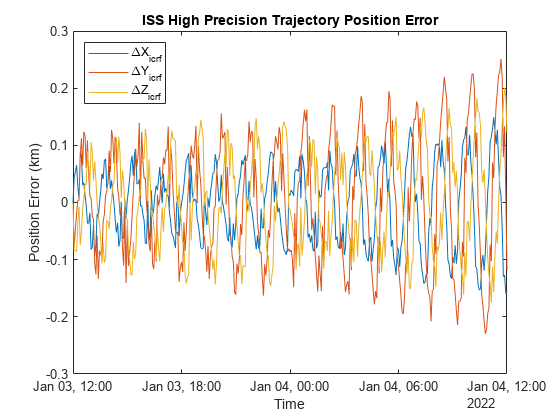
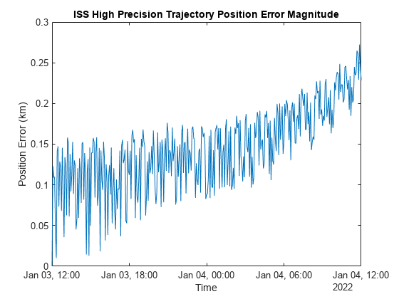
The maximum error between the simulation and the reference data over 24 hours is around 0.25km.
plot(iss.EphPosICRF.Time, vecnorm(iss.EphPosICRF.Data - iss.RefEphemeris.pos_eme2000.Position, 2, 2));
title("ISS High Precision Trajectory Position Error Magnitude");
xlabel("Time");
ylabel("Position Error (km)");
Compare High Precision Trajectory to Analytical Propagation
For comparison, add a new spacecraft to the satellite scenario using Two-Body-Keplerian propagation.
Convert initial position and velocity to orbital elements.
[iss.OrbEl.SemiMajorAxis, ...
    iss.OrbEl.Eccentricity, ...
    iss.OrbEl.Inclination, ...
    iss.OrbEl.RAAN, ...
    iss.OrbEl.ArgPeriapsis, ...
    iss.OrbEl.TrueAnomaly] =  ijk2keplerian(iss.X0_icrf*1e3, iss.V0_icrf*1e3);
Add a new ISS object to the scenario using Two-Body-Keplerian propagation.
iss.KeplerianOrbit.obj = satellite(scenario, iss.OrbEl.SemiMajorAxis, ...
    iss.OrbEl.Eccentricity, iss.OrbEl.Inclination, iss.OrbEl.RAAN, ...
    iss.OrbEl.ArgPeriapsis, iss.OrbEl.TrueAnomaly, ...
    OrbitPropagator="two-body-keplerian", ...
    Name="ISS Keplerian");
iss.KeplerianOrbit.obj.Orbit.LineColor = "magenta";
iss.KeplerianOrbit.obj.MarkerColor = "#8E3A59";
iss.KeplerianOrbit.obj.MarkerSize = "10";

Plot the maximum error for Two-Body-Keplerian propagation.
[iss.KeplerianOrbit.EphPosICRFData, ~, ...
    iss.KeplerianOrbit.TimeSteps] = states(iss.KeplerianOrbit.obj, CoordinateFrame="inertial");
iss.KeplerianOrbit.EphPosICRF = retime(timetable(iss.KeplerianOrbit.TimeSteps', iss.KeplerianOrbit.EphPosICRFData', VariableNames="Data"), ...
    iss.RefEphemeris.pos_eme2000.Time);
plot(iss.EphPosICRF.Time, iss.KeplerianOrbit.EphPosICRF.Data/1e3 - iss.RefEphemeris.pos_eme2000.Position);
title("ISS Two Body Keplerian Position Error");
xlabel("Time");
ylabel("Position Error (km)");
legend(["\DeltaX_{icrf}","\DeltaY_{icrf}","\DeltaZ_{icrf}"], Location="northwest");
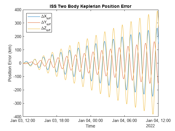
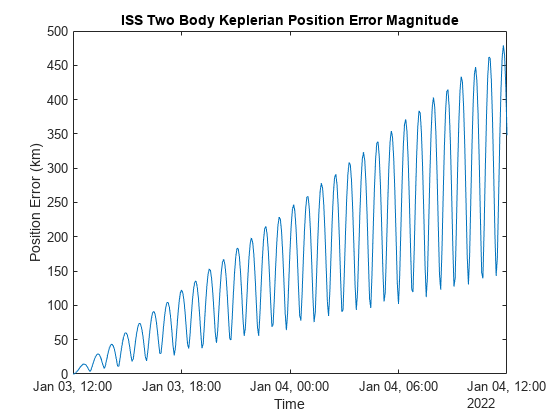
The maximum error between the Two-Body-Keplerian propagation and the reference data over 24 hours approaches exceeds 450km, compared to 0.25km for the high precision numerical propagation simulation.
plot(iss.EphPosICRF.Time, vecnorm(iss.KeplerianOrbit.EphPosICRF.Data/1e3 - iss.RefEphemeris.pos_eme2000.Position, 2, 2));
title("ISS Two Body Keplerian Position Error Magnitude");
xlabel("Time");
ylabel("Position Error (km)");
References
[1] NASA Open Data Portal - Trajectory Operations and Planning (TOPO), ISS_COORDS_2022-01-03 Public Distribution File - https://data.nasa.gov/Space-Science/ISS_COORDS_2022-01-03/ffwr-gv9k
[2] Vallado, David. Fundamentals of Astrodynamics and Applications, 4th ed. Hawthorne, CA: Microcosm Press, 2013.
See Also
Blocks
- Orbit Propagator Kepler (unperturbed) | Spherical Harmonic Gravity Model | NRLMSISE-00 Atmosphere Model
Objects
Select a Web Site
Choose a web site to get translated content where available and see local events and offers. Based on your location, we recommend that you select: United States.
You can also select a web site from the following list
Americas
- América Latina (Español)
- Canada (English)
- United States (English)
Europe
- Belgium (English)
- Denmark (English)
- Deutschland (Deutsch)
- España (Español)
- Finland (English)
- France (Français)
- Ireland (English)
- Italia (Italiano)
- Luxembourg (English)
- Netherlands (English)
- Norway (English)
- Österreich (Deutsch)
- Portugal (English)
- Sweden (English)
- Switzerland
- United Kingdom (English)
Asia Pacific
- Australia (English)
- India (English)
- New Zealand (English)
- 中国
- 日本Japanese (日本語)
- 한국Korean (한국어)