Detection of Known Signals with Coherent and Non-Coherent Receivers

This example discusses the detection of a deterministic signal in complex, white, Gaussian noise. A matched filter is used to take advantage of the processing gain. This situation is frequently encountered in radar, sonar and communication applications.

Overview

There are many different kinds of detectors available for use in different applications. A few of the most popular ones are the Bayesian detector, maximum likelihood (ML) detector and Neyman-Pearson (NP) detector. In radar and sonar applications, NP and its variation are the most popular choice since they can ensure the probability of false alarm ($$P_{fa}$$) to be at a certain level.

In this example, we limit our discussion to the scenario where the signal is deterministic, and the noise is white and Gaussian distributed. Both signal and noise are complex.

The example discusses the following topics and their interrelations: coherent detection, noncoherent detection, matched filtering and receiver operating characteristic (ROC) curves. This example mainly contains four parts. In the first part, we introduce the problem of single-dimensional signal detection using coherent receiver. We show that this problem is an NP detection problem and can be solved using a matched filter. In the following three parts, we present the variations of the NP detection problem to the cases of multi-dimensional signal detection, noncoherent detection, and noncoherent detection with pulse integration, respectively. The matched filter method is also extended in these three cases. The performance is calculated using Monte Carlo simulations and theoretical ROC curves.

Matched Filter

The received data is assumed to follow the model

$x=s+n.$

where $$s$$ is the signal and $$n$$ is the noise. Without losing the generality, we assume that the signal power is equal to 1 watt and the noise power is determined accordingly based on the signal to noise ratio (SNR). For example, for an SNR of 10 dB, the noise power, i.e., noise variance will be 0.1 watt.

A matched filter is often used at the receiver front end to enhance the SNR. From the discrete signal point of view, matched filter coefficients are simply given by the complex conjugated reversed signal samples.

When dealing with complex signals and noises, there are two types of receivers. The first kind is a coherent receiver, which assumes that both the amplitude and phase of the received signal are known. This results in a perfect match between the matched filter coefficients and the signal $$s$$. Therefore, the matched filter coefficients can be considered as the conjugate of $$s$$. The matched filter operation can then be modeled as

$$y=s^{H}x=s^H(s+n)=|s{|}^2+s^{H}n.$$

Note that although the general output $$y$$ is still a complex quantity, the signal is completely characterized by $$|s{|}^2$$, which is a real number and contained in the real part of $$y$$. Hence, the detector following the matched filter in a coherent receiver normally uses only the real part of the received signal. Such a receiver can normally provide the best performance. However, the coherent receiver is vulnerable to phase errors. In addition, a coherent receiver also requires additional hardware to perform the phase detection. For a noncoherent receiver, the received signal is modeled as a copy of the original signal with a random phase error. With a noncoherent received signal, the detection after the matched filter is normally based on the power or magnitude of the signal since you need both real and imaginary parts to completely define the signal.

Detector

The goal of a detector is to solve the following hypothesis testing problem:

$$\{\begin{array}{cc}{\mathcal{H}}_0,& x=n,\\ {\mathcal{H}}_1,& x=s+n,\end{array}$$

where $${\mathcal{H}}_0$$ is referred to as the null hypothesis and $${\mathcal{H}}_1$$ as the alternative hypothesis.

An ideal detector is the NP detector based on the NP decision rule that maximizes the probability of detection, $$P_d={\int }_{R}p(x|{\mathcal{H}}_1)dx$$, while limiting the probability of false alarm, $$P_{fa}={\int }_{R}p(x|{\mathcal{H}}_0)dx$$, at a specified level $$a$$, where $$p(x|{\mathcal{H}}_0)$$ is the likelihood function given $${\mathcal{H}}_0$$, $$p(x|{\mathcal{H}}_1)$$ is the likelihood function given $${\mathcal{H}}_1$$, and $$R=\{x:decide{\mathcal{H}}_1\}$$ is the decision region. The NP decision rule can be formulated as

$$\begin{array}{l}\max P_d\\ s.t.P_{fa}=a.\end{array}$$

The NP detector can be derived as a likelihood ratio test (LRT) as follows:

$$\frac{p(x|{\mathcal{H}}_1)}{p(x|{\mathcal{H}}_0)}\genfrac{}{}{0ex}{}{\genfrac{}{}{0ex}{}{{\mathcal{H}}_1}{>}}{\genfrac{}{}{0ex}{}{<}{{\mathcal{H}}_0}}{\gamma }_{LRT}.$$

In this NP situation, since the false alarm is caused by the noise alone, the threshold $${\gamma }_{LRT}$$ is determined by the noise to ensure the fixed $$P_{fa}$$.

The general form of the LRT shown above is often difficult to evaluate. In real applications, we often use an easy to compute quantity from the signal, i.e., sufficient statistic, to replace the ratio of two probability density functions. The sufficient statistics, $$z$$, is a function of the received data $$x$$:

$$z=T(x).$$

For example, the sufficient statistics, $$z$$, may be as simple as

$$z=|y|=|s^{H}x|.$$

Then, the simplified detector becomes

$$z\genfrac{}{}{0ex}{}{\genfrac{}{}{0ex}{}{{\mathcal{H}}_1}{>}}{\genfrac{}{}{0ex}{}{<}{{\mathcal{H}}_0}}\gamma ,$$

where $$\gamma$$ is the threshold to the sufficient statistic $$z$$, acting just like the threshold $${\gamma }_{LRT}$$ to the LRT detector. Therefore, the threshold is not only related to the probability distributions, but also depends on the choice of sufficient statistic.

Single-Dimensional Signal Detection Using Coherent Receiver

We will first explore an example of detecting a single-dimensional signal in noise.

Assume the signal has unit power and the SNR is 3 dB. Using a 100000-trial Monte-Carlo simulation, we generate the signal and noise as follows.

rstream = RandStream.create('mt19937ar','seed',2009);

Ntrial = 1e5;                                                     % number of Monte-Carlo trials
snrdb = 3;                                                        % received signal SNR in dB
snr = db2pow(snrdb);                                              % received signal SNR in linear scale
spower = 1;                                                       % signal power is 1
npower = spower/snr;                                              % noise power
namp = sqrt(npower/2);                                            % noise amplitude in each channel
s = ones(1,Ntrial);                                               % signal  
n = namp*(randn(rstream,1,Ntrial)+1i*randn(rstream,1,Ntrial));    % noise

Note that the noise is complex, white and Gaussian distributed.

If the received signal contains the target, it is given by

x = s + n;

Now, we do the LRT detection and examine the performance of the phased.LRTDetector. The LRT detector adopts the matched filter and coherent receiver for detection. The matched filter in this case is trivial, since the signal itself is a unit sample.

mf = 1;

The received signal after the matched filter is given by

$$y=s^{H}x.$$

y = mf'*x;

The sufficient statistic, i.e., the value used to compare to the detection threshold, for a coherent receiver is the real part of the received signal after the matched filter, i.e.,

$$z=real(y).$$

z = real(y);

Let's assume that we want to fix the $$P_{fa}$$ to 1e-3. Given the sufficient statistic, $$z$$, the decision rule becomes

$$z\genfrac{}{}{0ex}{}{\genfrac{}{}{0ex}{}{{\mathcal{H}}_1}{>}}{\genfrac{}{}{0ex}{}{<}{{\mathcal{H}}_0}}\gamma ,$$

where the threshold $$\gamma$$ is related to $$P_{fa}$$ as

$$\gamma =\eta \sqrt{{\sigma }^2{g}_{MF}},P_{fa}=\frac{1}{2}[1-erf\left(\eta \right)].$$

In the equation, $${\sigma }^2$$ is the noise power and $$g_{MF}$$ is the matched filter gain. Note that $$\gamma$$ is the threshold of the signal after the matched filter and $${\sigma }^2{g}_{MF}$$ represents the noise power after the matched filter. So, $$\eta =\frac{\gamma }{\sqrt{{\sigma }^2{g}_{MF}}}$$ can be considered as the ratio between the signal and noise magnitude, i.e., it is related to the signal to noise ratio (SNR). Since SNR is normally referred to as the ratio between the signal and noise power, considering the units of each quantity in this expression, we can see that

$$\eta =\sqrt{SN{R}_{thresh}}.$$

Given $$\gamma$$ is a threshold of the signal, $$SN{R}_{thresh}$$ can be considered as a threshold of the SNR. Therefore, the threshold equation can then be rewritten in the form of

$$P_{fa}=\frac{1}{2}[1-erf\left(\sqrt{SN{R}_{thresh}}\right)].$$

The required SNR threshold $$SN{R}_{thresh}$$ given a complex, white Gaussian noise for the LRT detector can be calculated using the npwgnthresh function as follows:

Pfa = 1e-3;
snrthreshold = db2pow(npwgnthresh(Pfa, 1,'coherent'));

Note that this threshold $$SN{R}_{thresh}$$, although also in the form of an SNR value, is different to the SNR of the received signal. The SNR threshold $$SN{R}_{thresh}$$ is a calculated value based on the desired detection performance, in this case the $$P_{fa}$$; while the received signal SNR is the physical characteristic of the signal determined by the propagation environment, the waveform, the transmit power, etc.

The signal detection threshold $$\gamma$$ can then be derived from this SNR threshold as

$$\gamma =\sqrt{{\sigma }^2{g}_{MF}}\cdot \sqrt{SN{R}_{thresh}}.$$

mfgain = mf'*mf;
threshold = sqrt(npower*mfgain*snrthreshold);

The detection is performed by comparing the sufficient statistics $$z$$ to the signal detection threshold $$\gamma$$. A successful detection occurs when the received signal passes the threshold, i.e., $$z>\gamma$$. The capability of the detector to detect a target is often measured by the $$P_d$$. In a Monte-Carlo simulation, $$P_d$$ can be estimated as the ratio between the number of times the signal passes the threshold and the number of total trials.

pd = sum(z>threshold)/Ntrial %#ok<NASGU>

pd = 0.1390

This workflow can be simplified using phased.LRTDetector, which uses the known signal $$s$$ and noise power $${\sigma }^2$$ for LRT detection.

lrt = phased.LRTDetector('DataComplexity','Complex',...
    'ProbabilityFalseAlarm',Pfa);

dresult = lrt(x,mf,npower);

pd = sum(dresult)/Ntrial %#ok<NASGU>

pd = 0.1390

On the other hand, a false alarm occurs when the detection shows that there is a target but there actually isn't one, i.e., the received signal passes the threshold when there is only noise present. The error probability of the detector to detect a target when there isn't one is given by the false alarm rate.

x = n;
y = mf'*x;
z = real(y);
pfa = sum(z>threshold)/Ntrial %#ok<NASGU>

pfa = 9.0000e-04

Alternatively, the false alarm rate can be obtained by

dresult = lrt(x,mf,npower);

pfa = sum(dresult)/Ntrial %#ok<NASGU>

pfa = 9.0000e-04

The resulting false alarm rate meets our requirement.

To see the relation among the received signal SNR, $$P_d$$ and $$P_{fa}$$ in a graph, we can plot the theoretical ROC curve using the rocsnr function for a received signal SNR value of 3 dB as

rocsnr(snrdb,'SignalType','NonfluctuatingCoherent','MinPfa',1e-4);

It can be seen from the figure that the measured $$P_d=0.1390$$ and $$P_{fa}=0.0009$$ obtained above for the received signal SNR value of 3 dB match a theoretical point on the ROC curve.

Multi-Dimensional Signal Detection Using Coherent Receiver

As discussed in the previous example, the threshold is determined based on $$P_{fa}$$. Therefore, as long as the threshold is chosen, the $$P_{fa}$$ is fixed, and vice versa. Meanwhile, one certainly prefers to have a higher probability of detection ($$P_d$$). One way to achieve that is to use multiple samples to perform the detection. For example, in the previous case, the SNR at a single-dimensional signal is 3 dB. If one can use multiple samples, then the matched filter can produce an extra gain in SNR and thus improve the performance. In practice, one can use a longer waveform that is a multi-dimensional signal to achieve this gain.

Assume that the waveform is now formed with a two-dimensional signal:

N = 2;
wf = ones(N,1).*exp(1i*2*pi*0.1*(0:N-1)');
mf = wf;

For a coherent receiver, the signal, noise and threshold are given by

s = wf*ones(1,Ntrial);
n = namp*(randn(rstream,N,Ntrial)+1i*randn(rstream,N,Ntrial));
snrthreshold = db2pow(npwgnthresh(Pfa, 1,'coherent'));
mfgain = mf'*mf;
threshold = sqrt(npower*mfgain*snrthreshold);

If the target is present

x = s + n;
y = mf'*x;
z = real(y);
pd = sum(z>threshold)/Ntrial %#ok<NASGU>

pd = 0.3940

Alternatively, we can estimate the probability of detection using the LRT detector.

release(lrt)

dresult = lrt(x,wf,npower);

pd = sum(dresult)/Ntrial %#ok<NASGU>

pd = 0.3940

If the target is absent

x = n;
y = mf'*x;
z = real(y);
pfa = sum(z>threshold)/Ntrial %#ok<NASGU>

pfa = 0.0010

Alternatively, we can estimate the probability of false alarm using the LRT detector.

dresult = lrt(x,wf,npower);

pfa = sum(dresult)/Ntrial %#ok<NASGU>

pfa = 0.0010

Notice that the signal SNR is improved by the matched filter.

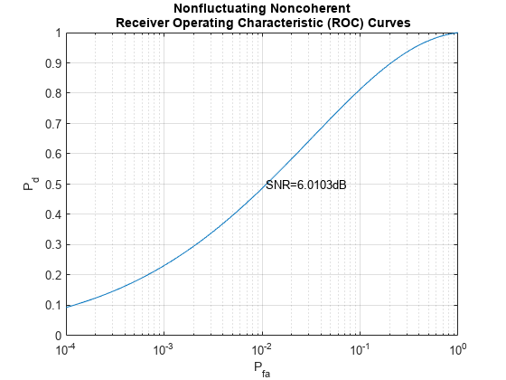
snr_new = snr*mfgain;
snrdb_new = pow2db(snr_new)

snrdb_new = 6.0103

Plot the ROC curve with this new SNR value.

rocsnr(snrdb_new,'SignalType','NonfluctuatingCoherent','MinPfa',1e-4);

One can see from the figure that the point given by $$P_{fa}$$ and $$P_d$$ falls right on the curve. The SNR corresponding to the ROC curve is the SNR at the output of the matched filter. The resulting $$P_{fa}$$ remains the same compared to the single-dimensional signal case. However, the extra matched gain improved the $$P_d$$ from 0.1390 to 0.3940.

Multi-Dimensional Signal Detection Using Noncoherent Receiver

In radar and sonar applications, the transmitted waveform $$s$$ is known but the received waveform can be distorted by the channel due to target reflection or propagation loss. In this case, the received data $$x$$ contains an unknown complex amplitude term, and the model of the data $$x$$ is defined as

$$x=\alpha s+n.$$

For example, consider the waveform $$s$$ is distorted by a random phase term:

x = s.*exp(1i*2*pi*rand(rstream,1,Ntrial)) + n;

The received signal after the matched filter is given by

$$y=s^{H}x.$$

y = mf'*x;

When the noncoherent receiver is used, the quantity used to compare with the threshold is the power (or magnitude) of the received signal after the matched filter. In this simulation, we choose the magnitude as the sufficient statistic, i.e.,

$$z=|y|.$$

z = abs(y);

Given the sufficient statistic, $$z$$, the decision rule becomes

$$z\genfrac{}{}{0ex}{}{\genfrac{}{}{0ex}{}{{\mathcal{H}}_1}{>}}{\genfrac{}{}{0ex}{}{<}{{\mathcal{H}}_0}}\gamma ,$$

where the threshold $$\gamma$$ is related to $$P_{fa}$$ as

$$P_{fa}=exp(-\frac{{\gamma }^2}{{\sigma }^2{g}_{MF}})=exp(-SN{R}_{thresh}).$$

The SNR threshold $$SN{R}_{thresh}$$ for the noncoherent receiver can be calculated using npwgnthresh as follows:

snrthreshold = db2pow(npwgnthresh(Pfa, 1,'noncoherent'));

The threshold, $$\gamma$$, is derived from $$SN{R}_{thresh}$$ as before.

threshold = sqrt(npower*mfgain*snrthreshold);

Again, $$P_d$$ can then be obtained using

pd = sum(z>threshold)/Ntrial %#ok<NASGU>

pd = 0.2318

Note that this resulting $$P_d$$ is inferior to the performance we get from a coherent receiver.

The above noncoherent receiver can be theoretically derived by the phased.GLRTDetector under linear deterministic signal model $$\alpha s$$, where $$\alpha$$ is treated as an unknown parameter and the signal $$s$$ is treated as the observation matrix. The hypothesis testing problem can be reduced to

$$\{\begin{array}{cc}{\mathcal{H}}_0,& 1\cdot \alpha =0,\\ {\mathcal{H}}_1,& 1\cdot \alpha \ne 0.\end{array}$$

Thus, the above workflow can be simplified using phased.GLRTDetector, which uses the observation matrix $$s$$, the augmented linear equality constraint matrix $$[1,0]$$, and noise power $${\sigma }^2$$ for GLRT detection.

glrt = phased.GLRTDetector('DataComplexity','Complex',...
    'ProbabilityFalseAlarm',Pfa,'NoiseInputPort',true);

dresult = glrt(x,[1 0],wf,npower);

pd = sum(dresult)/Ntrial %#ok<NASGU>

pd = 0.2318

For the target absent case, the received signal contains only noise. We can calculate the $$P_{fa}$$ using Monte-Carlo simulation as

x = n;
y = mf'*x;
z = abs(y);
pfa = sum(z>threshold)/Ntrial %#ok<NASGU>

pfa = 0.0012

Alternatively, the false alarm rate can be obtained by

dresult = glrt(x,[1 0],wf,npower);

pfa = sum(dresult)/Ntrial %#ok<NASGU>

pfa = 0.0012

The ROC curve for a noncoherent receiver is plotted as

rocsnr(snrdb_new,'SignalType','NonfluctuatingNoncoherent','MinPfa',1e-4);

We can see that the performance of the noncoherent receiver detector is inferior to that of the coherent receiver.

Multi-Dimensional Signal Detection Using Noncoherent Receiver with Pulse Integration

Radar and sonar applications frequently use pulse integration to improve the detection performance. If the receiver is coherent, the pulse integration is just concatenating waveforms over multiple pulses for matched filtering. Thus, the SNR improvement is linear when one uses the coherent receiver. If one integrates 10 pulses, then the SNR at the output of the concatenated matched filter is improved 10 times. For a noncoherent receiver, the relationship is not that simple. The following example shows the use of pulse integration with a noncoherent receiver.

Assume an integration of 2 pulses. Then, construct the received signal and apply the matched filter to it.

PulseIntNum = 2;
Ntotal = PulseIntNum*Ntrial;
s = mf*exp(1i*2*pi*rand(rstream,1,Ntotal));
n = sqrt(npower/2)*...
    (randn(rstream,N,Ntotal)+1i*randn(rstream,N,Ntotal));

If the target is present

x = s + n;
y = mf'*x;
y = reshape(y,Ntrial,PulseIntNum);

One can integrate the pulses using either of two possible approaches. Both approaches are related to the approximation of the modified Bessel function of the first kind, which is encountered in modeling the LRT of the noncoherent detection process using multiple pulses. The first approach is to sum $$|y{|}^2$$ across the pulses, which is often referred to as a square law detector. The second approach is to sum together $$|y|$$ from all pulses, which is often referred to as a linear detector. For small SNR, square law detector is preferred while for large SNR, using linear detector is advantageous. We use square law detector in this simulation. However, the difference between the two kinds of detectors is normally within 0.2 dB.

For this example, choose the square law detector, which is more popular than the linear detector. To perform the square law detector, one can use the pulsint function. The function treats each column of the input data matrix as an individual pulse. The pulsint function performs the operation of

$$z=\sqrt{|y_1{|}^2+\cdots +|y_L{|}^2}$$

over $$L$$ pulses.

z = pulsint(y,'noncoherent');

The relation between the threshold $$\gamma$$ and the $$P_{fa}$$, given this new sufficient statistics, $$z$$, is given by

$$P_{fa}=1-I(\frac{{\gamma }^2/({\sigma }^2{g}_{MF})}{\sqrt{L}},L-1)=1-I(\frac{SN{R}_{thresh}}{\sqrt{L}},L-1).$$

where

$$I(u,K)={\int }_0^{u\sqrt{K+1}}\frac{e^{-\tau }{\tau }^K}{K!}d\tau$$

is Pearson's form of the incomplete gamma function and $$L$$ is the number of pulses used for pulse integration. Using a square law detector, one can calculate the SNR threshold $$SN{R}_{thresh}$$ involving the pulse integration using the npwgnthresh function as before.

snrthreshold = db2pow(npwgnthresh(Pfa,PulseIntNum,'noncoherent'));

The resulting threshold for the sufficient statistics, $$z$$, is given by

threshold = sqrt(npower*mfgain*snrthreshold);

The probability of detection is obtained by

pd = sum(z>threshold)/Ntrial

pd = 0.5260

Then, calculate the $$P_{fa}$$ when the received signal is noise only using the noncoherent detector with 2 pulses integrated.

x = n;
y = mf'*x;
y = reshape(y,Ntrial,PulseIntNum);
z = pulsint(y,'noncoherent');
pfa = sum(z>threshold)/Ntrial

pfa = 9.7000e-04

To plot the ROC curve with pulse integration, one has to specify the number of pulses used in integration in rocsnr function:

rocsnr(snrdb_new,'SignalType','NonfluctuatingNoncoherent',...
    'MinPfa',1e-4,'NumPulses',PulseIntNum);

Again, the point given by $$P_{fa}$$ and $$P_d$$ falls on the curve. The SNR in the ROC curve specifies the SNR at the output of the matched filter from one pulse.

Such an SNR value can also be obtained from $$P_d$$ and $$P_{fa}$$ using Albersheim's equation. The result obtained from Albersheim's equation is just an approximation, but is fairly good over frequently used $$P_{fa}$$, $$P_d$$ and pulse integration length $$L$$.

Note: Albersheim's equation has many assumptions, such as the target is nonfluctuating (Swirling case 0 or 5), the noise is complex, white Gaussian, the receiver is noncoherent and the linear detector is used for detection (square law detector for nonfluctuating target is also ok).

To calculate the necessary single pulse SNR to achieve a certain $$P_d$$ and $$P_{fa}$$ with pulse integration length $$L$$, use the Albersheim function as

snr_required = albersheim(pd,pfa,PulseIntNum)

snr_required = 6.0278

This calculated required SNR value matches the new SNR value of 6 dB.

To see the improvement achieved in $$P_d$$ by pulse integration, plot the ROC curve when there is no pulse integration used.

rocsnr(snrdb_new,'SignalType','NonfluctuatingNoncoherent',...
    'MinPfa',1e-4,'NumPulses',1);

From the figure, one can see that without pulse integration, $$P_d$$ can only be around 0.2318 with $$P_{fa}$$ at 1e-3. With 2-pulse integration, as illustrated in the above Monte Carlo simulation, for the same $$P_{fa}$$, the $$P_d$$ is around 0.53.

Summary

This example shows how to simulate and perform different detection techniques using MATLAB®. The example illustrates the relationship among several frequently encountered variables in signal detection, namely, probability of detection ($$P_d$$), probability of false alarm ($$P_{fa}$$) and signal to noise ratio (SNR). In particular, the example calculates the performance of the detector using Monte-Carlo simulations and verifies the results of the metrics with the receiver operating characteristic (ROC) curves.

There are two SNR values we encounter in detecting a signal. The first one is the SNR of a single data sample. This is the SNR value appeared in a ROC curve plot. A point on ROC gives the required single sample SNR necessary to achieve the corresponding $$P_d$$ and $$P_{fa}$$. However, it is NOT the SNR threshold used for detection. Using the Neyman-Pearson (NP) decision rule, the SNR threshold, the second SNR value we see in the detection, is determined by the noise distribution and the desired $$P_{fa}$$ level. Therefore, such an SNR threshold indeed corresponds to the $$P_{fa}$$ axis in a ROC curve. If we fix the SNR of a single sample, as depicted in the above ROC curve plots, each point on the curve will correspond to a $$P_{fa}$$ value, which in turn translates to an SNR threshold value. Using this particular SNR threshold to perform the detection will then result in the corresponding $$P_d$$.

Note that an SNR threshold may not be the threshold used directly in the actual detector. The actual detector normally uses an easy to compute sufficient statistic quantity to perform the detection. Thus, the true threshold has to be derived from the aforementioned SNR threshold accordingly so that it is consistent with the choice of sufficient statistics.

When perform detection using only a single-dimensional signal, the resulting $$P_d$$ is fairly low and there is no processing gain achieved by the matched filter. To improve $$P_d$$ and to take advantage of the processing gain of the matched filter, we can use a longer waveform with multi-dimension, or pulse integration of multiple pulses of the received signal. The example illustrates the relation among $$P_d$$, $$P_{fa}$$, ROC curve and Albersheim's equation. This example also shows the relation among matched filter, coherent receiver, noncoherent receiver, LRT detector, and GLRT detector. The performance is calculated using Monte Carlo simulations and theoretical ROC curves.

Reference

[1] Steven M. Kay, Fundamentals of Statistical Signal Processing, Detection Theory, 1998

[2] Mark A. Richards, Fundamentals of Radar Signal Processing, Third edition, McGraw-Hill Education, 2022.