Vehicle Path Tracking Using Stanley Controller
From the series: Improving Your Racecar Development
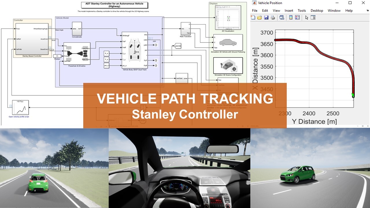
Learn how to implement a Stanley controller for path tracking and the steps to take to control the path of an autonomous vehicle. Create waypoints using the Driving Scenario Designer app, and build a path- tracking model in Simulink® using Automated Driving Toolbox™ and Vehicle Dynamics Blockset™. See how you can visualize and compare the vehicle’s trajectory in 2D, 3D, and bird’s-eye view. Discover how to simulate a three degrees-of-freedom (3DOF) vehicle driving around an oval track that is specified by waypoints in the Follow Waypoints Around Oval Track documentation example. You can find the example models used in this video on the MATLAB Central File Exchange.
Published: 4 Aug 2021
Hello, everyone. Welcome to MATLAB and Simulink Racing Lounge. Today, we are going to talk about vehicle path tracking using Stanley Controller. And to talk about this, I have my colleague David Barnes, so David, why don't you introduce yourself?
Hey everybody. My name is David Barnes. I'm an engineer here in the engineering development group. I had the opportunity to work with Veer on this new project, where we're going to be looking at vehicle path tracking using Stanley controller.
Awesome, so David, why don't you show us some pictures, some videos, what we're going to see today.
Awesome, yeah. We'll go ahead and get started here. As you can see, we're going to have this car that's going to be exiting this highway off towards the right. As it's going to be sweeping, you see the vehicle being able to be controlled, both in its longitudinal and its lateral direction, as it's going through making some velocity sweeps. And we'll be following it as it goes back off towards the left as well.
So let's move to the agenda, and see what all we are going to cover today.
So we're going to look at the Stanley Controller itself. We'll take a look at its implementation, starting with generation of waypoints, and then moving on to actually implementing this, and building the models in Simulink, and of course doing all of these visualizations of the vehicle motion. And of course, we'll wrap up with some key takeaways for you all.
OK, so basically, we are going to focus mostly on the implementation part.
Yes. For those of you that don't know, the Stanley Controller has been around for a little while, and it's actually a path tracking algorithm. It was actually first used in real life in the Stanford racing team in the DARPA GRAND Challenge, and it's using and computing the steering wheel angle to follow a reference trajectory. We don't want to get into all the details of the derivation of this, but you can feel free to look at the reference here.
So basically, we have taken this formula from the reference that we have provided. And if you want to know more, you can refer to the paper.
So let's take a look at how this is actually implemented with the products. We're first going to start by generating waypoints in Driving Scenario Designer, then we'll move over into actually calculating some of the reference input parameters for our Simulink model, using a MATLAB live script. Then we'll actually build the vehicle and the controller model in Simulink. And finally, wrap up with visualizing all of this motion in bird's eye view, two dimensional plots, as well as the 3D environment using Unreal. Let's go to MATLAB and get started.
So let's first open up the Driving Scenario Designer, coming over here to the apps. I happen to have it In the start, but you can also search for it up here at the top. Driving Scenario Designer. We can get started by actually adding the road to the scenario canvas. Once we click on the Add Route button, we're able to just click waypoints. And as we're clicking through, we're going to be adding these as our road centers, and then heading enter button.
Driving Scenario will generate our road for us. We can go ahead and add an actor, and there's several options for you to choose from, including cars, pedestrians, or bicycles. We'll get started today with just adding a car to our starting area. We'll start by clicking on there to add our actor as its initial point. And then we can right click on it, and add forward waypoints. Once we're here, we can continue to click through on these road centers, and show the path that we want this vehicle to follow. Again hitting Enter, we'll save these waypoints, and we can visualize this within Driving Scenario Designer by hitting the run button.
As you can see, this vehicle oscillates back and forth following with these waypoints, and if you want to, you can change the vehicle's constant velocity here. We can save this as a scenario file. And this is going to save a ton of information from the scenario, including the road information, information about the actors, as well as any sensors you might have added. Once we save this, we can then call this from a live script. Now that we've saved our scenario file, and exported it from Driving Scenario Designer, we've saved it here as simple track. We can now use this in our live scripts.
The script that we have here is going to set up everything for our Simulink model. The first thing we'll do is add in some of the images that we use in the model, but then we're actually going to load in scene files. We're going to grab the waypoints from the references that are in there from the actor's specifications, and then we'll define those waypoints, based on the x and the y values as the first and the second column. Then, we need to give some of the blocks the initial position of the vehicle. So we can describe the first element in those reference vectors.
Some of the other information that we'll need is going to include the distance vector to see how far along the vehicle is moving along its path. So after calculating that, we will also linearize and smooth this data, so that it's nice and clean for our Simulink model. We'll also need to calculate the angle for it. This is using the a tan 2d, which is the four quadrant tangent calculation, and it's going to output all the values in degrees. And then again, smoothing this, and grabbing some initial values for the yaw angle.
Next, we'll also need to create the direction vector. This is just simple vector of 1's, because it's always moving forward. In the chance that you have a scenario where you are moving forwards and backwards, you can use negative 1 for those directions. Then, we're going to calculate the curvature, using just a simple curvature calculation function down the bottom. For our x in our y values, and we're all ready to get started with our model.
OK, David. Thanks for covering that. So it means that it is not necessary that the user has to grab the waypoints from the Driving Scenario Designer, even if they are having some kind of test data. So they can have the values over here, and then they can go through the same procedure.
Exactly. Awesome. With all of these values calculated, we can go ahead and go to the model. Now that we've got the model open, we can go ahead, and take a look at the different components for it. The first, starting over on the left, is the reference data.
We went through and calculated all of these different values as a function of the vehicle's distance. So as we input the vehicle's velocity, we're just going to simply integrate that to see how far along its path it is. And then we'll be outputting from these simple lookup tables, the x values, y values, angle, as well as its curvature and direction.
Now that we have all of those states, we can actually pass this in to the Stanley Controller. So using the automated driving toolbox implementation of the Stanley controller, it's relatively simple for you to get started with the kinematic bicycle model. All that you need to do is change the gains for your forward motion as well as your reverse, and then give it some specifications about your vehicle, such as its total wheel base, as well as the maximum steering angle that you want for your controller.
So yeah, and I think the advantage in using Stanley Controller is that we do have an upper bound. For here, we are using a maximum steering angle, which we have kept 35. So, yeah. Simple as that.
Now that we have everything defined and our Controller ready, all we have to do is pull these signals into the three degree of freedom vehicle body to do all of these calculations. For this simulation, we're using just a constant velocity that will change. Let's go ahead and see how the simulation runs. As you can see the vehicle is following the path fairly well. As it's moving through, you'll have a little bit of cross-track error as it's going, but it will slowly start to match over the course of some time.
So now that our controller is working fairly well, let's see what happens if we increase the velocity a little bit. So we can go ahead and increase this velocity from 8 meters per second to, let's say, 12 meters per second. Just a little bit faster. Now when we run the simulation, let's see how our controller responds. After the model compiles, we'll see that the vehicle starts off doing fairly well, in terms of its track but--
OK, I can see some deviation.
Yes. Quite a bit from this controller. And as you can see, as the curvature starts to increase for the waypoints, the vehicle definitely has a little bit of spin off as it goes in its different directions.
But we can actually make this a whole lot better by switching the type of Stanley implementation that we're using. And that's going to be moving and switching the actual type of model that's used in the Stanley Controller. This is going to be taking and moving from this vehicle model of a kinematic bicycle model, which is a little bit unstable in terms of its system, to the dynamic model.
So with these new values, we actually have new ports that become available. Starting from the top, one of the first ones is curvature, which we fortunately already have calculated using the reference data. So I'll go ahead and connect that here. The next is going to be the current yaw rate, which we already get out of our three degree of freedom dual track model, which is this value r. I can just right-click the signal, and drag it in. And then the next is the current steering rate, and so we'll be able to use that by passing it into a unit delay block, and get this connected in.
So this is basically to avoid the algebraic loop?
Exactly. Now that we have our model ready to go, I'm going to turn off stimulation pacing now that we've seen it a few times, and we'll go ahead and let this model run. As you see, the model runs quite quickly without simulation pacing--
Ah, OK.
And we have fantastic values in terms of how our vehicle's responding to this high velocity, as well as the curves.
So yeah David, this looks great, and just a question. So the vehicle parameters that you defined when you selected the dynamics model in the lateral controller. So are those also defined in the vehicle body 3DOF dual track?
Yes, they certainly are. You want to make sure that all those values match as you're making sure that your vehicle is there. And you can find these hidden into these different options here. So for your vehicle parameters, you'll have those matching here, such as your vehicle mass in those distances to the to the axle.
Is there a way where we can compare all these vehicles and have a proper Visualization.
Yes, we certainly do, and that's going to be using the Simulink data inspector. So we've already saved this from some previous runs, and we can go ahead and grab that. And what we can see from here is based off of the different parameters that we had, such as the type of model that's used in the Stanley Controller, as well as those gains, we can actually press play down here at the bottom, and watch and see these values as a function of time, as well as their positions x and y.
So that's a great tool, because it is showing the x, y comparison, and also the state and command comparison.
Awesome. Now that we've seen a fairly simple model, let's see what happens when we increase some of the fidelity for our models. Well, we're adding in higher fidelity by modeling the powertrain and the driveline in this block right here. By going in, we have created a simple powertrain model, as well as drivelines, braking systems, as well as adding in the brakes and wheels subsystem.
And so David, if you can click on the brakes and wheels. So this tire has been taken from the vehicle dynamics blocks.
Correct, yes. Now that we've had this powertrain model, we actually have a little bit of a change to our vehicle dynamics block. Instead of having a constant input, or maybe a changing input for your velocity, we're now modeling the velocity changes, based on the forces on the front and the rear axles.
This means that we'll take our calculated vehicle velocity, and change this into a distance. This will allow us to then be able to control the velocity using a Stanley-based controller. Based on the position of the vehicle, similar to how we have our other states, we're now going to have a velocity to control for, in our Stanley-based controller. It's going to be a combined longitudinal and lateral controller. So let's take a look.
In here we have our same Stanley Controller for our lateral dynamics. That's going to be taking into account our states, and it's going to be using the dynamic bicycle model, so that we have this nice, clean control. But we're also going to have the longitudinal control, here, based off of the current velocity and the direction of the vehicle.
This is also very similar, where we're using this simple controller with a proportional and an interval gain, and with a specified sample time. We're also going to use vehicle parameters, like the maximum and minimum longitudinal acceleration and deceleration rates.
So David, this is basically to track the velocity reference.
Exactly. So now we'll be able to control the vehicle's position, as well as how fast it's going.
OK, in the last model, we were just having constant velocity. Now we have a varying velocity, a reference velocity for this.
Correct.
So that's awesome, that's a good addition to the model.
Yes. So now let's see where this velocity profile is actually coming from. It's in the script here that's hyperlinked in this link, and feel free to take a look at this script to see how we're using the trapezoidal rule to calculate and smooth out a velocity based on of its position. And then, going back to the model, we've added some additional ways that we can visualize this vehicle.
We still have our 2D visualization with that x y plotter that's available in some of the other vehicle dynamic block sets examples. As well as adding in the 3D visualization in Unreal using just these two blocks. There's also the opportunity to use the bird's eye scope using the block that's here, and is readily available using the bird's eye scope, up here at the top ribbon.
Now that we have the bird's eye scope set up, we're ready to run the simulation. By pressing run either here or in the simulation tab, we can watch all of our different visualization options. And here we go. Now we have the vehicle moving along its path, similar to the video that we saw earlier.
Now that the simulation has finished, we can actually see that the circles that were previously uniform, now have sections that are scrunched up and more spread apart, and this is based on the vehicle's velocity changing as a function of path. So now we're able to see that across our simulation, the Stanley controllers were able to fairly well keep both the longitudinal and the lateral states of the vehicle intact.
OK, that's great.
These were using the automated driving toolboxes implementation, but there's also some available in the vehicle dynamics block set.
So David, can you show the block in the library browser where we can find it in the vehicle dynamics blocks?
We certainly can. Opening up the library browser, we can actually see where the original blocks came from, here out of the Automated Driving Toolbox. They're coming here out of your vehicle control. And then you have your lateral Stanley Controller, as well as your longitudinal one.
Or, going all the way down to the vehicle dynamics block set, we can see that these are available here in your vehicle scenarios, and then moving into the different driver models that are available. You'll have these available as a lateral driver, a longitudinal one, or available as combined in the Predictive driver as well.
So David, do we have any example of where we can see the implementation of this predictive driver, where we can select the option for the Stanley Controller?
Yes, we do. Actually, shipping in 21a, there's a new example reference application that I think would be perfect. As you can see this is a very similar layout to the model we have before, where we have some reference values coming from here, whereas instead of our calculations, this oval track reference, where we can see the implementation of the predictive driver, here in this model. Opening up this combined longitudinal and lateral driver, we see that actually the lateral control type can be either Stanley or predictive.
So we are also defining the same parameters that we defined in the previous block. So David, can you show where we are defining those parameters?
Certainly. So over here under the reference control, we can see that the Stanley value still has these gains associated with it, and we're still also passing in vehicle parameters, here shown as a part of the structure of the vehicle.
So David, do we have any visualization in this one, because I can see a subsystem in the visualization, so can you go inside that and show the viewers what extra we got?
Exactly. So similar to what we had, there's the 3D visualization using Unreal. There's also a brand new GG plotter that's available for the simulation. Let's go ahead and run the model, and see what this looks like.
As you can see, we're going to have a little bit more information about the vehicle forces that are involved in the velocity on the tires, but we also now have this new GG diagram, which shows as the vehicle goes around the track, how these accelerations are actually occurring.
OK, that's awesome, David. Because I think that the GG plotter addition in this model is very much relevant to the racing teams. So that's great, David. I think we have seen all the models. So can we go to the key takeaways of this video?
Yeah, so today, we've gotten to see quite a few different things. But first off, was showing how we can smooth some of these reference input parameters, and that's going to be a very important step for you, as you're going to continue developing your own models, so that you have really good tracking. And a lot of that has to come in to the second point, which is based on higher velocities and varying curvatures, combining these lateral and longitudinal dynamics are really going to give you better path tracking results, based on that nice, smooth data.
And MATLAB and Simulink do provide you a whole lot of algorithms and tools for doing these different parts of the process, from generating some of these waypoints, to building the vehicle model and the controllers, and also visualizing these in different levels of fidelity in different environments.
Yeah, thanks David, and for all the viewers, if you want to contact us, you can contact us at racinglounge@mathworks.com, and feel free to join our Facebook group, where we keep on sharing the latest technical resources, and even updates regarding our upcoming webinars. And for more videos and tutorials, you can visit the student tutorials and videos website. So with this, we've come to the end of the video. Thanks David, that was a great presentation, and we covered a lot of things like implementation of Stanley Controllers using MATLAB and Simulink.
Thank you, so much.
Download Code and Files
Related Products
Learn More


웹사이트 선택
번역된 콘텐츠를 보고 지역별 이벤트와 혜택을 살펴보려면 웹사이트를 선택하십시오. 현재 계신 지역에 따라 다음 웹사이트를 권장합니다: United States
또한 다음 목록에서 웹사이트를 선택하실 수도 있습니다.
미주
- América Latina (Español)
- Canada (English)
- United States (English)
유럽
- Belgium (English)
- Denmark (English)
- Deutschland (Deutsch)
- España (Español)
- Finland (English)
- France (Français)
- Ireland (English)
- Italia (Italiano)
- Luxembourg (English)
- Netherlands (English)
- Norway (English)
- Österreich (Deutsch)
- Portugal (English)
- Sweden (English)
- Switzerland
- United Kingdom (English)