Differential Equations and Linear Algebra, 1.2: The Calculus You Need

From the series: Differential Equations and Linear Algebra

Gilbert Strang, Massachusetts Institute of Technology (MIT)

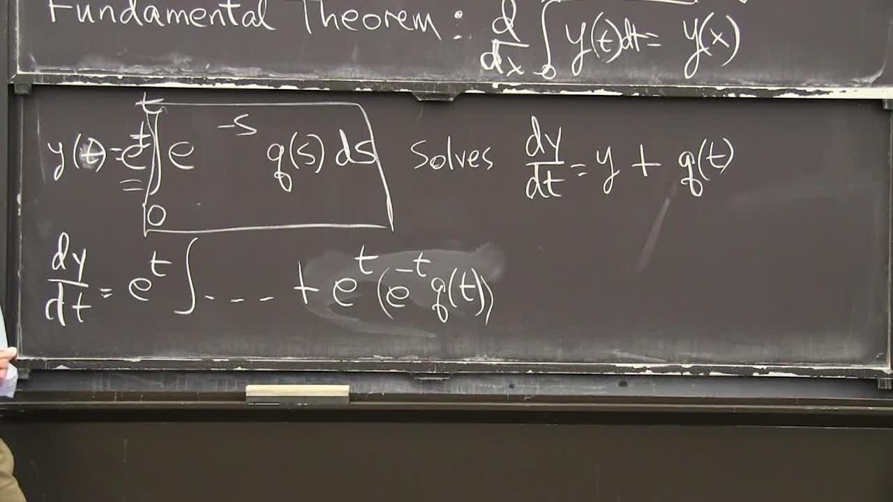
The sum rule, product rule, and chain rule produce new derivatives from the derivatives of xⁿ, sin(x) and e^x. The Fundamental Theorem of Calculus says that the integral inverts the derivative.

Video Transcript

OK well, here we're at the beginning. And that I think it's worth thinking about what we know. Calculus. Differential equations is the big application of calculus, so it's kind of interesting to see what part of calculus, what information and what ideas from calculus, actually get used in differential equations. And I'm going to show you what I see, and it's not everything by any means, it's some basic ideas, but not all the details you learned. So I'm not saying forget all those, but just focus on what matters.

OK. So the calculus you need is my topic. And the first thing is, you really do need to know basic derivatives. The derivative of x to the n, the derivative of sine and cosine. Above all, the derivative of e to the x, which is e to the x. The derivative of e to the x is e to the x. That's the wonderful equation that is solved by e to the x. Dy dt equals y.

We'll have to do more with that. And then the inverse function related to the exponential is the logarithm. With that special derivative of 1/x. OK. But you know those. Secondly, out of those few specific facts, you can create the derivatives of an enormous array of functions using the key rules.

The derivative of f plus g is the derivative of f plus the derivative of g. Derivative is a linear operation. The product rule fg prime plus gf prime. The quotient rule. Who can remember that?

And above all, the chain rule. The derivative of this-- of that chain of functions, that composite function is the derivative of f with respect to g times the derivative of g with respect to x. That's really-- that it's chains of functions that really blow open the functions or we can deal with.

OK. And then the fundamental theorem. So the fundamental theorem involves the derivative and the integral. And it says that one is the inverse operation to the other. The derivative of the integral of a function is this.

Here is y and the integral goes from 0 to x I don't care what that dummy variable is. I can-- I'll change that dummy variable to t. Whatever. I don't care. To show the dummy variable.

The x is the limit of integration. I won't discuss that fundamental theorem, but it certainly is fundamental and I'll use it. Maybe that's better. I'll use the fundamental theorem right away.

So-- but remember what it says. It says that if you take a function, you integrate it, you take the derivative, you get the function back again. OK can I apply that to a really-- I see this as a key example in differential equations. And let me show you the function I have in mind. The function I have in mind, I'll call it y, is the interval from 0 to t.

So it's a function of t then, time, It's the integral of this, e to the t minus s. Some function. That's a remarkable formula for the solution to a basic differential equation.

So with this, that solves the equation dy dt equals y plus q of t. So when I see that equation and we'll see it again and we'll derive this formula, but now I want to just use the fundamental theorem of calculus to check the formula. What as we created-- as we derive the formula-- well it won't be wrong because our derivation will be good. But also, it would be nice, I just think if you plug that in, to that differential equation it's solved.

OK so I want to take the derivative of that. That's my job. And that's why I do it here because it uses all the rules. OK to take that derivative, I notice the t is appearing there in the usual place, and it's also inside the integral. But this is a simple function.

I can take e to the t-- I'm going to take e to the t out of the-- outside the integral. e to the t. So I have a function t times another function of t.

I'm going to use the product rule and show that the derivative of that product is one term will be y and the other term will be q. Can I just apply the product rule to this function that I've pulled out of a hat, but you'll see it again. OK so it's a product of this times this. So the derivative dy dt is-- the product rule says take the derivative of -- that is e to the --.

Plus, the first thing times the derivative of the second. Now I'm using the product rule. It just-- you have to notice that e to the t came twice because it is there and its derivative is the same. OK now, what's the derivative of that? Fundamental theorem of calculus.

We've integrated something, I want to take its derivative, so I get that something. I get e to the minus tq of t. That's the fundamental theorem. Are you good with that?

So let's just look and see what we have. First term was exactly y. Exactly what is above because when I took the derivative of the first guy, the f it didn't change it, so I still have y. What have I-- what do I have here? E to the t times e to the minus t is one.

So e to the t cancels e to the minus t and I'm left with q of t Just what I want. So the two terms from the product rule are the two terms in the differential equation. I just think as you saw the fundamental theorem was needed right there to find the derivative of what's in that box, is what's in those parentheses. I just like that the use of the fundamental theorem.

OK one more topic of calculus we need. And here we go. So it involves the tangent line to the graph. This tangent to the graph.

So it's a straight line and what we need is y of t plus delta t. That's taking any function, maybe you'd rather I just called the function f. A function at a point a little beyond t, is approximately the function at t plus the correction because it-- plus a delta f, right? A delta f.

And what's the delta f approximately? It's approximately delta t times the derivative at t. That-- there's a lot of symbols on that line, but it expresses the most basic fact of differential calculus. If I put that f of t on this side with a minus sign, then I have delta f. If I divide by that delta t, then the same rule is saying that this is approximately df dt.

That's a fundamental idea of calculus, that the derivative is quite close. At the point t-- the derivative at the point t is close to delta f divided by delta t. It changes over a short time interval. OK so that's the tangent line because it starts with that's the constant term. It's a function of delta t and that's the slope.

Just draw a picture. So I'm drawing a picture here. So let me draw a graph of-- oh there's the graph of e to the t. So it starts up with slope 1. Let me give it a little slope here.

OK the tangent line, and of course it comes down here Not below. So the tangent line is that line.

That's the tangent line. That's this approximation to f. And you see as I-- here is t equals 0 let's say. And here's t equal delta t. And you see if I take a big step, my line is far from the curve.

And we want to get closer. So the way to get closer is we have to take into account the bending. The curve is bending. What derivative tells us about bending?

That is delta t squared times the second derivative. One half. It turns out a one half shows in there. So this is the term that changes the tangent line, to a tangent parabola. It notices the bending at that point. The second derivative at that point.

So it curves up. It doesn't follow it perfectly, but as well-- much better than the other. So this is the line. Here is the parabola. And here is the function. The real one.

OK. I won't review the theory there that it pulls out that one half, but you could check it. Now finally, what if we want to do even better? Well we need to take into account the third derivative and then the fourth derivative and so on, and if we get all those derivatives then, all of them that means, we will be at the function because that's a nice function, e to the t. We can recreate that function from knowing its height, its slope, its bending and all the rest of the terms.

So there's a whole lot more-- Infinitely many terms. That one over two-- the good way to think of one over two, one half, is one over two factorial, two times one. Because this is one over n factorial, times t to the nth, pretty small, times the nth derivative of the function. And keep going.

That's called the Taylor series named after Taylor. Kind of frightening at first. It's frightening because it's got infinitely many terms. And the terms are getting a little more comp-- For most functions, you really don't want to compute the nth derivative.

For e to the t, I don't mind computing the nth derivative because it's still e to the t, but usually that's-- this isn't so practical. -- very practical. Tangent parabola, quite practical. Higher order terms, less-- much less practical.

But the formula is beautiful because you see the pattern, that's really what mathematics is about patterns, and here you're seeing the pattern in the higher, higher terms. They all fit that pattern and when you add up all the terms, if you have a nice function, then the approximation becomes perfect and you would have equality.

So to end this lecture, approximate to equal provided we have a nice function. And those are the best functions of mathematics and exponential is of course one of them. OK that's calculus. Well, part of calculus. Thank you.

Other Resources

Read about differential equations and linear algebra

Learn more about Gilbert Strang

Series: Differential Equations and Linear Algebra

Introduction